Vector Indexing in Production: HNSW vs. DiskANN vs. IVF-PQ Architecture, Memory Footprint, and Search Economics

Scaling vector search beyond prototype deployments exposes a fundamental tension across three competing constraints: retrieval recall, query latency, and memory footprint. In high-dimensional representation spaces, exact k-nearest neighbor search via brute-force flat scans requires $O(N \cdot d)$ floating-point operations per query. For a corpus of 100 million 1536-dimensional FP32 embeddings, a single flat search pass requires scanning 614.4 GB of uncompressed data, creating unacceptable latency and memory bandwidth saturation.

Approximate Nearest Neighbor (ANN) indexing structures trade bounded recall loss for sub-linear search time. Production search platforms and retrieval-augmented generation (RAG) pipelines rely on three dominant indexing paradigms: pure in-memory proximity graphs (HNSW), inverted file clustering with product quantization (IVF-PQ), and disk-hybrid graph traversal with compressed routing (DiskANN). Each architectural choice imposes specific operational trade-offs across DRAM sizing, disk I/O characteristics, build times, and incremental update mechanics.

1. Hierarchical Navigable Small World (HNSW): Graph Topologies in DRAM

Introduced by Malkov and Yashunin (2018), Hierarchical Navigable Small World (HNSW) graphs remain the standard baseline for low-latency, high-recall vector search when entire datasets fit inside host memory.

Algorithmic Mechanics

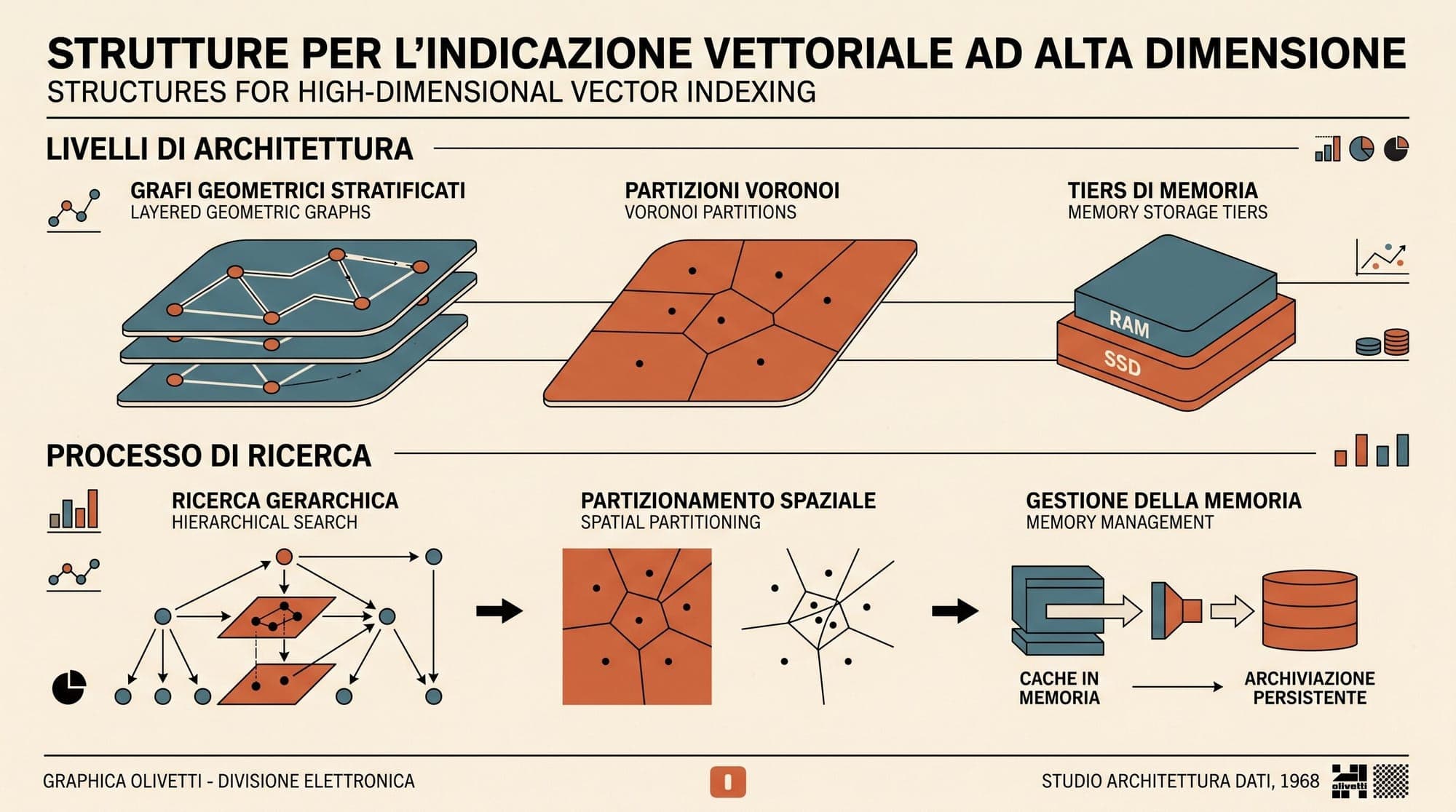
HNSW structures high-dimensional vector spaces into a multi-layer geometric graph analogous to a probabilistic skip-list:

1. Layer Assignment: Each inserted vector is assigned a maximum layer $l$ drawn from an exponential decay distribution:

$$l = \lfloor -\ln(\text{unif}(0, 1)) \cdot m_L \rfloor$$ where $m_L = 1/\ln(M)$. Higher layers are sparse and contain long-range navigational links. Layer 0 contains all vectors and forms a dense proximity graph.

1. Top-Down Routing: Search starts at a global entry point at top layer $L$. The query executes greedy routing: evaluating candidate neighbors and hopping to the closest node until a local minimum is reached.
2. Beam Search at Layer 0: The algorithm drops down layer by layer using the entry point found in the layer above. Upon reaching layer 0, the search expands from greedy routing to a priority-queue beam search bounded by the parameter efSearch.

Layer 2 (Sparse):    [Node A] ------------------------------> [Node F]
                         \                                       \
Layer 1 (Medium):    [Node A] ---------> [Node C] ----------> [Node F]
                         \                 \                     \
Layer 0 (Dense):     [Node A] <-> [Node B] <-> [Node C] <-> ... <-> [Node F]

Production Trade-Offs

• Latency and Recall: HNSW consistently delivers sub-2ms p95 latencies with 98% to 99% recall@10 on 1536-dimensional OpenAI embeddings and 768-dimensional BGE embeddings.
• Incremental Ingestion: New vectors can be inserted concurrently without invalidating the global graph. The insertion procedure routes to layer 0, identifies candidate neighbors via beam search bounded by efConstruction, and creates bidirectional edges using heuristic pruning.
• DRAM Overhead: HNSW stores raw vector arrays alongside adjacency lists containing $M$ integer pointers (typically 16 to 64 connections per node) across all layers. For 1536-dimensional FP32 vectors (6,144 bytes each) with $M=32$, graph connectivity metadata adds 256 to 512 bytes per point. Total DRAM consumption reaches 6.5 GB to 7.0 GB per million vectors.

For datasets exceeding 50 million to 100 million vectors, hosting pure HNSW graphs entirely in DRAM becomes economically prohibitive for enterprise search clusters.

2. Inverted File with Product Quantization (IVF-PQ): Subspace Compression

Formalized by Jégou, Douze, and Schmid (2011) and widely popularized by FAISS, IVF-PQ combines space partitioning with aggressive lossy vector compression to minimize memory consumption.

Algorithmic Mechanics

IVF-PQ operates as a two-stage coarse-fine indexing pipeline:

1. Inverted File Partitioning (IVF): The dataset is clustered into $K$ Voronoi cells using k-means (typically $K = 4096$ to $65536$ centroids). Each vector is assigned to its closest centroid $C_i$, and the index stores residual vectors:

$$r = v - C_i$$

1. Product Quantization (PQ): The residual vector space of dimension $d$ is decomposed into $m$ orthogonal sub-vectors of dimension $d/m$. For each sub-space, k-means generates $k^* = 256$ sub-centroids. Each sub-vector is replaced by an 8-bit (1-byte) index pointing to its nearest sub-centroid.

Original Vector (1536d FP32: 6,144 bytes)
  │
  ├──> Assigned to Centroid K (Voronoi Cell) -> Store Residual r = v - C_k
  │
  └──> Split r into m=64 Sub-Vectors (24 dims each)
         │  Sub-vector 1 -> Codebook Index (1 byte)
         │  Sub-vector 2 -> Codebook Index (1 byte)
         │  ...
         └── Sub-vector 64 -> Codebook Index (1 byte)
  │
Quantized Code: 64 bytes total (98.9% DRAM reduction)

Asymmetric Distance Computation (ADC)

During query execution, the unquantized query vector $q$ computes full-precision Euclidean or inner-product distances to the coarse centroids. The search selects the top nprobe Voronoi lists to scan.

For each selected list, the query precomputes a lookup table containing the distance from its sub-vectors to all 256 sub-centroids across all $m$ sub-spaces. Calculating distance to any quantized vector in the list requires only $m$ table lookups and byte additions:

$$D(q, v) \approx \sum_{j=1}^m \text{LUT}_j[\text{code}_j(v)]$$

No floating-point multiplications are executed during the candidate scan.

Production Trade-Offs

• Memory Efficiency: For 1536-dimensional vectors, setting $m=64$ reduces the vector footprint from 6,144 bytes to 64 bytes plus minimal centroid overhead. One million vectors occupy roughly 70 MB of RAM instead of 6.1 GB.
• Recall Degradation: Quantization introduces structural distortion. Real-world 1-recall@10 for IVF-PQ typically peaks between 82% and 92%, falling short of graph-based indexes on difficult out-of-distribution queries.
• Centroid Drift: As the underlying embedding distribution changes over time, fixed k-means centroids lose partitioning efficiency. IVF-PQ requires periodic offline rebuilds or background clustering recalculations to prevent severe recall drops.

3. DiskANN and Vamana Graphs: SSD Traversal with In-Memory Routing

Published by Subramanya et al. at Microsoft Research (NeurIPS 2019), DiskANN eliminated the assumption that high-recall graph indexes must reside entirely in volatile memory.

Algorithmic Mechanics

DiskANN introduces the single-layer Vamana graph, built using an aggressive distance-pruning algorithm called RobustPrune.

Unlike HNSW, which builds multiple hierarchical layers, Vamana builds a single flat graph. During index construction, RobustPrune selects edges using a parameter $\alpha \ge 1$ (typically $\alpha = 1.2$). An edge between candidate $p$ and neighbor $n$ is retained only if:

$$\text{dist}(p, n) < \alpha \cdot \text{dist}(n', n) \quad \forall n' \in \text{Edges}(p)$$

This rule explicitly favors long-range navigational edges with diverse directional angles over tightly clustered redundant short edges. The resulting graph maintains a low diameter and short search paths while residing on a single flat structure.

                [Host Memory (RAM)]
  ┌──────────────────────────────────────────────┐
  │ 1-Byte/2-Byte Quantized Vectors (PQ/RaBitQ) │
  │ Greedy Search Routes Query to Local Minima   │
  └──────────────────────┬───────────────────────┘
                         │ Asynchronous I/O (io_uring)
                         ▼
             [NVMe Solid-State Drive]
  ┌──────────────────────────────────────────────┐
  │ Sector-Aligned 4KB/8KB Graph Blocks:         │
  │ • Full-Precision FP32/FP16 Vectors           │
  │ • Vamana Adjacency Lists (Out-degree R=64)   │
  └──────────────────────────────────────────────┘

Hybrid Two-Tier Search Execution

DiskANN splits the retrieval workload between DRAM and fast NVMe storage:

1. Compressed In-Memory Routing: A heavily compressed representation of all vectors (e.g., 1-byte product quantized codes or 1-bit RaBitQ codes) resides in DRAM.
2. Greedy Traversal Without Disk Reads: Search starts at a pre-calculated medoid node. The query traverses the in-memory quantized graph using beam search, executing 10 to 30 graph hops without issuing a single disk I/O request.
3. Asynchronous Disk Verification: Once the beam reaches candidate nodes close to the query target, DiskANN issues parallel asynchronous I/O read requests (using Linux io_uring or libaio) to fetch raw uncompressed vectors and true graph adjacency lists stored in sector-aligned 4KB NVMe blocks.
4. Reranking: Full-precision distances are computed from the fetched SSD blocks to produce the final top-k response.

Production Trade-Offs

• Billion-Scale Density: DiskANN indexes and serves 1 billion 128-dimensional to 1536-dimensional vectors on a single workstation with 64 GB RAM and a commodity NVMe SSD, achieving >95% 1-recall@1 with 4ms to 8ms query latency. Pure HNSW would require 4 TB to 6 TB of DRAM distributed across a costly multi-node cluster.
• I/O Dependency: DiskANN requires high-throughput NVMe SSDs with high random 4KB read IOPS (minimum 500k to 1M IOPS). Performance degrades sharply on network-attached storage or legacy SATA SSDs.
• Tail Latency Sensitivity: Under high concurrent multi-tenant throughput, NVMe queue depth saturation can push p99 latencies from 5ms up to 25ms.

4. Production Architectural Comparison

+----------------------+----------------------+----------------------+----------------------+
| Feature / Metric     | HNSW (In-Memory)     | IVF-PQ (Quantized)   | DiskANN (Vamana)     |
+----------------------+----------------------+----------------------+----------------------+
| Storage Residence    | 100% Host DRAM       | 100% Host DRAM       | NVMe SSD + RAM Cache |
| Memory (1M 1536d)    | ~6.5 GB - 7.0 GB     | ~70 MB - 120 MB      | ~100 MB RAM + 6.2GB  |
| 1-Recall@10 Ceiling  | 98.0% - 99.5%        | 84.0% - 92.0%        | 95.0% - 98.5%        |
| Query Latency (p95)  | 1.0 ms - 2.5 ms      | 2.0 ms - 6.0 ms      | 4.0 ms - 8.0 ms      |
| Build Throughput     | ~5k - 15k vec/s      | ~25k - 50k vec/s     | ~3k - 8k vec/s       |
| Incremental Inserts  | Real-time concurrent | Append to cell/drift | Staged merge buffers |
| Cost (100M Vectors)  | ~$5,000 - $8,000/mo  | ~$300 - $600/mo      | ~$400 - $800/mo      |
| Core Bottleneck      | DRAM capacity & cost | Quantization noise   | Random NVMe IOPS     |
+----------------------+----------------------+----------------------+----------------------+

Key operational trade-offs across these architectures:

• HNSW provides the lowest latency and highest recall ceiling, but requires linear DRAM scaling that becomes cost-prohibitive beyond tens of millions of high-dimensional vectors.
• IVF-PQ achieves the lowest memory footprint in pure DRAM environments, but suffers from lower recall ceilings and requires clustering re-calibration when vector distributions shift.
• DiskANN bridges the gap by maintaining near-graph recall (95%+) while moving 95% of the memory footprint to NVMe SSDs, drastically lowering total cost of ownership for 100M+ vector workloads.

5. Architectural Selection Guidelines

Selecting the right vector indexing architecture depends on corpus scale, query latency budgets, and budget constraints:

                        ┌───────────────────────────────┐
                        │   Total Vector Corpus Size?   │
                        └───────────────┬───────────────┘
                                        │
                 ┌──────────────────────┴──────────────────────┐
                 ▼                                             ▼
        [ < 10M Vectors ]                             [ > 10M Vectors ]
                 │                                             │
                 ▼                                             ▼
      ┌─────────────────────┐                     ┌────────────────────────┐
      │   Pure HNSW (RAM)   │                     │ Latency SLA < 3ms p95? │
      │  Sub-2ms, 99% Recall│                     └───────────┬────────────┘
      └─────────────────────┘                                 │
                                               ┌──────────────┴──────────────┐
                                               ▼                             ▼
                                            [ YES ]                        [ NO ]
                                               │                             │
                                               ▼                             ▼
                                    ┌──────────────────────┐      ┌──────────────────────┐
                                    │ Quantized HNSW (RAM) │      │   DiskANN (NVMe+RAM) │
                                    │ (HNSW + SQ8/RaBitQ)  │      │ 95%+ Recall, 5ms p95 │
                                    └──────────────────────┘      └──────────────────────┘

1. Deploy Pure HNSW When:

• Dataset scale is under 10 million vectors.
• P99 latency SLAs are strict (under 3ms).
• Real-time continuous insertion and immediate search availability are required without background batch re-indexing.

1. Deploy Quantized HNSW (HNSW + SQ8 / RaBitQ) When:

• Dataset scale ranges between 10 million and 100 million vectors.
• Low latency is critical, but raw FP32 DRAM costs exceed infrastructure budgets.
• Scalar Quantization (SQ8) or binary hypercube quantization (RaBitQ) preserves 96%+ recall while reducing vector memory by 75%.

1. Deploy DiskANN When:

• Dataset scale spans 100 million to multiple billions of vectors.
• Workloads run on single-node or compact multi-node systems with local NVMe PCIe Gen4/Gen5 storage.
• A 4ms to 8ms query latency profile is acceptable in exchange for a 5x to 10x reduction in cloud hosting bills.

1. Deploy IVF-PQ / Partitioned Quantization When:

• Workloads require massive batch filtering over pre-filtered relational partitions.
• Embeddings are heavily clustered and memory must remain strictly bounded in multi-tenant environments.

Sources

• Malkov, Yu. A., and D. A. Yashunin. "Efficient and robust approximate nearest neighbor search using Hierarchical Navigable Small World graphs." IEEE TPAMI / arXiv:1603.09320 (2018).
• Subramanya, Suhas Jayaram, Devvrit, Rohan Kadekodi, Ravishankar Krishnaswamy, and Harsha Vardhan Simhadri. "DiskANN: Fast Accurate Billion-point Nearest Neighbor Search on a Single Node." Advances in Neural Information Processing Systems (NeurIPS 2019).
• Jégou, Hervé, Matthijs Douze, and Cordelia Schmid. "Product Quantization for Nearest Neighbor Search." IEEE Transactions on Pattern Analysis and Machine Intelligence (TPAMI 2011).
• Microsoft Research. "DiskANN: Graph-based approximate nearest neighbor search." GitHub Repository.
• Faiss: A library for efficient similarity search and clustering of dense vectors. Meta AI Research.