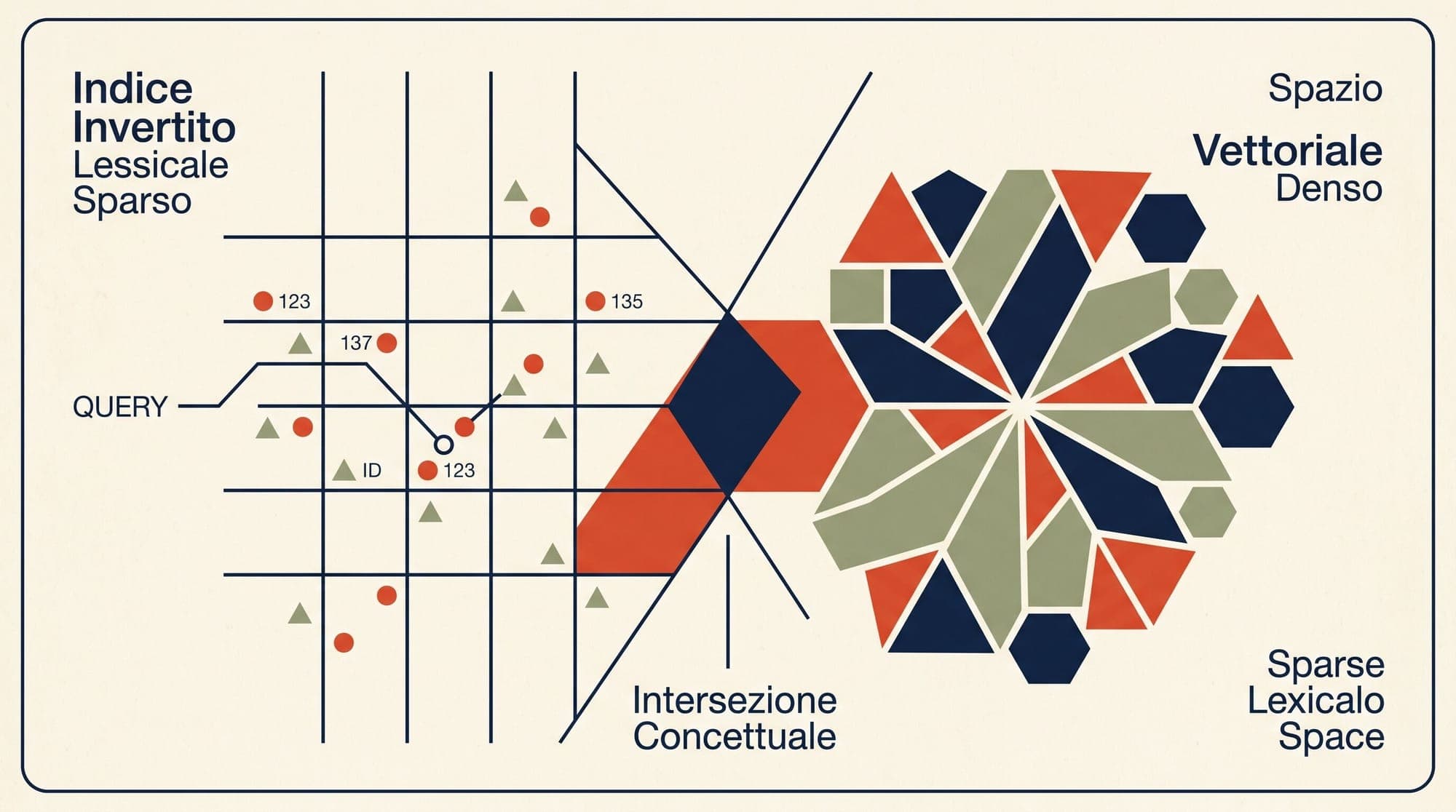
Sparse-Dense Hybrid Retrieval in Production: Learned Lexical Weights, SPLADE vs. BGE-M3, Inverted Index Pruning, and Serving Economics

Modern Retrieval-Augmented Generation (RAG) and enterprise search architectures increasingly encounter the operational limits of pure dense vector search. Dense bi-encoders project text passages into continuous latent spaces (typically 768 to 3,072 dimensions). While dense representations excel at conceptual matching and paraphrasing, they systematically struggle with exact keyword precision, rare alphanumeric tokens, product SKUs, and domain-specific jargon. Furthermore, serving dense vectors at scale requires graph-based Approximate Nearest Neighbor (ANN) indices such as Hierarchical Navigable Small World (HNSW), which consume massive amounts of uncompressed RAM.

Traditional lexical search algorithms like BM25 offer exact term matching with lightweight, CPU-efficient inverted index posting lists. However, BM25 operates on exact token overlaps, failing when users query synonyms or related terms not explicitly present in the corpus.

Learned sparse retrieval bridges this architectural divide. By using transformer encoders to project documents and queries into high-dimensional vocabulary spaces with learned token importance and automated query expansion, models such as SPLADE (Formal et al., 2021) and BGE-M3 (Chen et al., 2024) deliver lexical precision, semantic expansion, and the hardware efficiency of inverted indices.

The Architecture of Learned Sparse Representations

Learned sparse models repurpose the masked language modeling (MLM) output layer of transformer encoders. Instead of compressing a sequence into a single dense vector, the model computes a sparse weight vector over the entire tokenizer vocabulary $V$ .

For an input sequence $d = (t_1, t_2, \dots, t_N)$ , the transformer generates contextualized token representations $h_1, h_2, \dots, h_N \in \mathbb{R}^d$ . For each token position $i$ and each vocabulary item $j \in V$ , the model predicts a relevance score:

$s_{i,j} = \text{transform}(h_i)_j + b_j$

In SPLADE, the sequence-level weight for vocabulary term $j$ is calculated via max-pooling across all token positions, followed by a log-saturation transform:

$w_j = \max_{i \in d} \log(1 + \text{ReLU}(s_{i,j}))$

To ensure that the resulting vector remains sparse rather than generating non-zero weights for all 30,000+ vocabulary dimensions, training incorporates sparsity-inducing regularizers. The most common approaches include:

L1 Regularization: Penalizes the sum of absolute term weights $\lambda \sum_{j \in V} |w_j|$ .
FLOPS Regularization: Penalizes the expected number of operations during retrieval by computing the square of mean term activations across batch documents: $\lambda_{flops} \sum_{j \in V} \left( \frac{1}{|B|} \sum_{d \in B} w_{d,j} \right)^2$.

This dynamic produces sparse vectors where typically only 100 to 300 dimensions out of the full vocabulary have non-zero values.

Input: "transformer memory footprint"
Vocabulary Dimension: 30,522 (BERT WordPiece)

Non-Zero Activations:
  "transformer":  2.41
  "memory":       2.15
  "footprint":    1.89
  "vram":         1.42  <-- Learned expansion (not in raw input)
  "gpu":          1.18  <-- Learned expansion
  "attention":    0.95  <-- Learned expansion
  "cache":        0.82  <-- Learned expansion
  [All other 30,515 dimensions = 0.0]

SPLADE vs. BGE-M3: Architectural Comparison

Two primary learned sparse paradigms dominate production deployments: dedicated sparse encoders (SPLADE v2, Efficient-SPLADE) and unified multi-functional encoders (BGE-M3).

While SPLADE uses an MLM prediction head with explicit FLOPS regularization to maximize zero-weights, BGE-M3 trains a unified representation where a linear layer over hidden states outputs token weights directly for the 250k multilingual vocabulary. BGE-M3 allows engineers to generate dense embeddings, sparse lexical weights, and late-interaction multi-vectors from a single forward pass, eliminating redundant inference pipelines.

Inverted Index Traversal and Pruning Strategies

Because learned sparse embeddings are mathematically equivalent to weighted bag-of-words vectors, they can be stored and searched using inverted indices rather than dense vector graphs.

Inverted Index Traversal and Pruning Architecture

In an inverted index, each dimension in the vocabulary corresponds to a posting list containing tuples of (document_id, weight). The relevance score between query $q$ and document $d$ is the dot product of their sparse vectors:

$\text{Score}(q, d) = \sum_{t \in q \cap d} w_{q,t} \cdot w_{d,t}$

However, because neural expansion adds more active terms per document than raw BM25, posting lists can grow long, potentially degrading query latency. Production search systems use three primary pruning mechanisms:

1. Offline Index Pruning (Thresholding)

During ingestion, any term weight falling below an absolute threshold $\epsilon$ (e.g., $w_{d,j} < 0.1$ ) is truncated before writing to the posting list. This drops 40% to 60% of low-confidence expansion tail terms with negligible loss in retrieval recall (NDCG@10 degradation < 0.5%).

2. Weak AND (WAND) Algorithm

Originally developed by Broder et al. (2003), WAND tracks the maximum possible contribution $U_t$ of each term's posting list. During query execution over terms $(t_1, \dots, t_k)$ , WAND sorts posting lists by current document pointer and accumulates upper bounds:

$\sum_{m=1}^p U_{t_m} \ge \theta$

If the accumulated upper bound cannot exceed the current $k$ -th best document threshold $\theta$ , candidate documents are skipped without computing full dot products.

3. Block-Max WAND (BMW)

Ding and Suel (2011) refined WAND by partitioning posting lists into fixed-size blocks (e.g., 64 or 128 postings) and caching the maximum score $U_{b,t}$ per block. Block-Max WAND allows search engines like Lucene, OpenSearch, Vespa, and Qdrant to skip entire blocks of non-competitive documents, reducing posting list evaluation time by 3x to 5x compared to standard linear traversal.

Serving Economics: Sparse vs. Dense Infrastructure

The infrastructure trade-offs between sparse and dense indexing are substantial across memory footprint, CPU utilization, and latency.

For large-scale corpora (10M+ documents), maintaining dense vectors in memory becomes a dominant cost driver. A 10-million document corpus indexed in HNSW at 1,536 dimensions requires approximately 70 GB of uncompressed RAM solely for index structures. The corresponding learned sparse index compressed with SIMD-PForDelta requires under 10 GB and can serve queries directly from memory-mapped disk pages.

Hybrid Integration Topologies in Production RAG

In production RAG systems, learned sparse retrieval is rarely used in total isolation. Instead, it serves as the lexical backbone of hybrid retrieval architectures.

Architecture 1: Linear Interpolation (Single Datastore)

Modern vector databases (e.g., Qdrant, Milvus, Vespa, Azure AI Search) support native sparse-dense hybrid search. Both dense vectors and sparse lexical weights are stored in the same document record. At query time, the system computes both distances and combines them linearly:

$\text{FinalScore}(q, d) = \alpha \cdot \text{DenseScore}(q, d) + (1 - \alpha) \cdot \text{SparseScore}(q, d)$

Tuning $\alpha \in [0.4, 0.7]$ consistently outperforms pure dense search on cross-domain benchmarks such as BEIR, preventing semantic drift on specific identifiers while preserving topical generalization.

Architecture 2: Two-Phase Fusion with Reciprocal Rank Fusion (RRF)

When dense and sparse indices reside in separate systems (e.g., Pinecone/Milvus for dense and OpenSearch/Elasticsearch for sparse), scores exist on different numerical scales. Reciprocal Rank Fusion (RRF) merges rank positions without requiring score normalization:

$\text{RRFScore}(d) = \sum_{m \in \{\text{dense}, \text{sparse}\}} \frac{1}{k + r_m(d)}$

Where $k \approx 60$ acts as a ranking stabilizer. Top- $N$ candidates from RRF are subsequently routed to a cross-encoder reranker (e.g., BGE-Reranker-Large or Cohere Rerank 3) for final precision scoring.

Common Production Pitfalls and Mitigations

Query Expansion Latency Overheads: Running a full BERT forward pass to compute query token expansions can add 15ms to 30ms on CPU. In latency-sensitive setups, deploy query encoders on GPU or use distilled variants like Efficient-SPLADE-Query, which prune the query expansion head to fewer than 20 active non-zero terms.
Vocabulary Incompatibilities: Sparse representations are strictly bound to their tokenizer vocabulary. Upgrading an embedding model from a 30k vocabulary to a 250k vocabulary requires a full corpus re-encoding and re-indexing.
Document Length Skew: Long documents can activate thousands of expansion terms if max-pooling is evaluated over several thousand tokens without length-normalization penalties. Splitting documents into 256-word chunks before encoding prevents posting list bloat.