Direct Preference Optimization: Mathematical Derivation, Implicit Reward Formulation, and the Mechanics of RL-Free Alignment

Aligning autoregressive large language models with human preferences has traditionally relied on Reinforcement Learning from Human Feedback (RLHF). In the standard formulation popularized by InstructGPT and related post-training regimes, alignment requires a multi-stage pipeline: supervised fine-tuning (SFT), training a separate reward model on pairwise comparison data, and optimizing the policy model against that reward model using Proximal Policy Optimization (PPO).

While effective, classical RLHF introduces severe systems-level complexity and numerical instability. Training with PPO requires orchestrating four distinct neural networks in accelerator memory simultaneously: the active policy, the frozen reference policy, the value (critic) network, and the reward model. Furthermore, online rollout generation during training creates significant GPU memory bandwidth bottlenecks and high variance in policy gradient estimation.

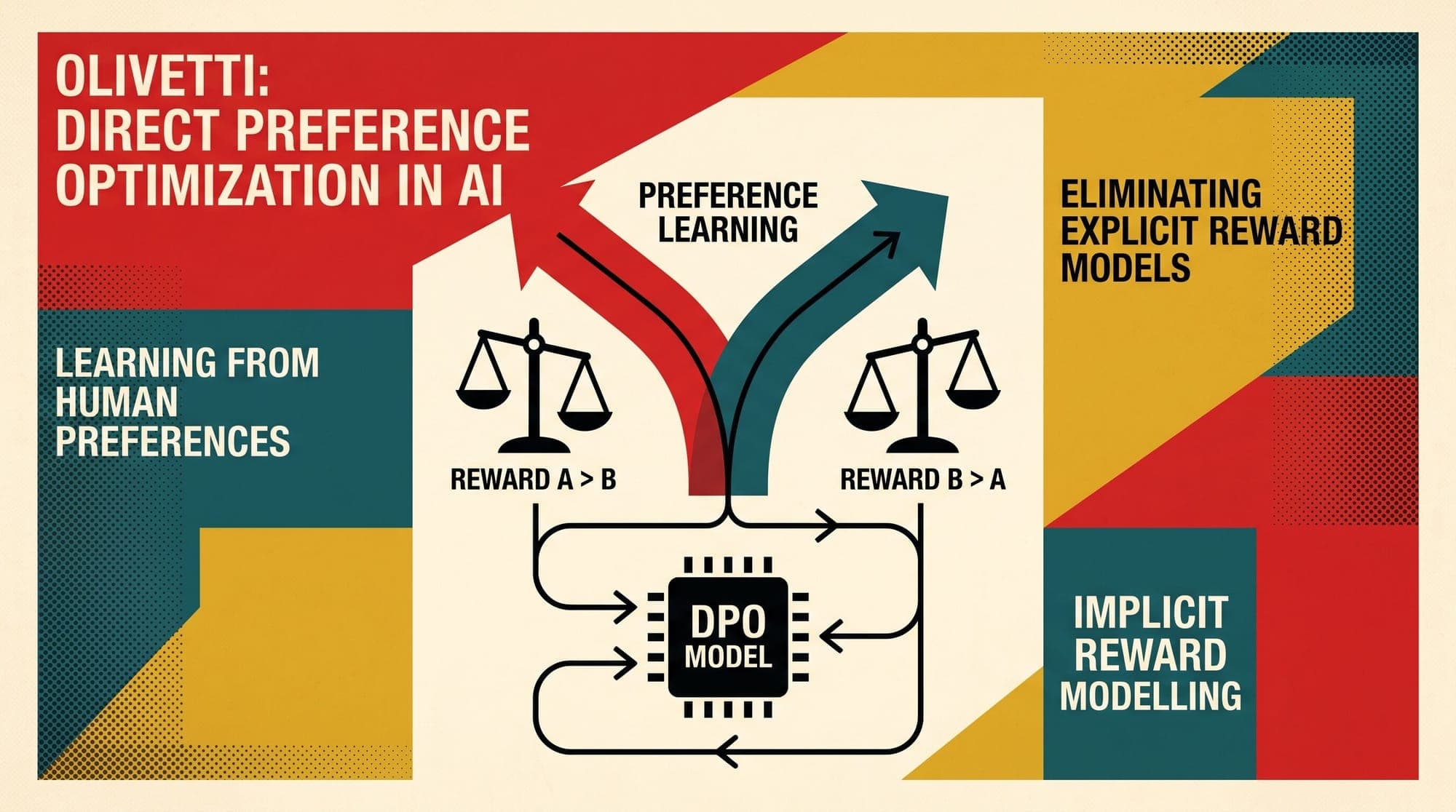
In 2023, researchers introduced Direct Preference Optimization (DPO), demonstrating that the constrained reinforcement learning objective used in RLHF can be solved in closed form. By algebraically reparameterizing the latent reward function directly in terms of the optimal policy and a reference policy, DPO eliminates the need for explicit reward modeling and dynamic policy sampling altogether.

The Classical RLHF Optimization Problem

To understand DPO, one must first examine the mathematical objective of standard RLHF. Given a prompt dataset $\mathcal{D}$ and a reference policy $\pi_{\text{ref}}$ (typically the SFT model checkpoint), the goal is to find a parameterized policy $\pi_\theta$ that maximizes the expected scalar reward while remaining close to the reference policy under Kullback-Leibler (KL) divergence.

The formal optimization problem is defined as:

$$\max_{\pi} \mathbb{E}_{x \sim \mathcal{D}, y \sim \pi(y|x)} [r(x, y)] - \beta D_{\text{KL}}(\pi(y|x) \parallel \pi_{\text{ref}}(y|x))$$

Here, $r(x, y)$ represents the ground-truth latent reward function, $D_{\text{KL}}$ is the forward KL divergence between the policy and reference distributions, and $\beta > 0$ is a regularization parameter controlling the trade-off between maximizing reward and penalizing drift from the reference distribution.

Expanding the expectation and the KL divergence term reveals the per-prompt objective:

$$\max_{\pi} \mathbb{E}_{x \sim \mathcal{D}} \left[ \sum_{y} \pi(y|x) r(x, y) - \beta \sum_{y} \pi(y|x) \log \frac{\pi(y|x)}{\pi_{\text{ref}}(y|x)} \right]$$

subject to the probability simplex constraint:

$$\sum_{y} \pi(y|x) = 1 \quad \text{and} \quad \pi(y|x) \ge 0 \quad \forall y$$

In classical RLHF, because $r(x, y)$ is unobservable, practitioners approximate it by fitting a parameterized reward model $r_\phi(x, y)$ on a dataset of pairwise human preferences $\mathcal{D} = \{(x^{(i)}, y_w^{(i)}, y_l^{(i)})\}_{i=1}^N$, where $y_w$ denotes the preferred (winning) response and $y_l$ denotes the dispreferred (losing) response.

Under the Bradley-Terry (1952) preference model, the probability that a human prefers $y_w$ over $y_l$ given prompt $x$ is parameterized as:

$$P(y_w \succ y_l \mid x) = \sigma(r(x, y_w) - r(x, y_l)) = \frac{1}{1 + \exp(-(r(x, y_w) - r(x, y_l)))}$$

The reward model parameters $\phi$ are trained via negative log-likelihood:

$$\mathcal{L}_R(\phi) = - \mathbb{E}_{(x, y_w, y_l) \sim \mathcal{D}} \left[ \log \sigma(r_\phi(x, y_w) - r_\phi(x, y_l)) \right]$$

Once $r_\phi$ is trained, PPO (Schulman et al., 2017) is used to update the policy $\pi_\theta$ against $r_\phi(x, y) - \beta \log \frac{\pi_\theta(y|x)}{\pi_{\text{ref}}(y|x)}$. This requires generating responses on the fly, calculating token-level Generalized Advantage Estimations (GAE), and fitting a separate value head.

Deriving the Closed-Form Optimal Policy

The core theoretical breakthrough of DPO begins by analyzing the global optimum of the KL-regularized objective without introducing an external reward model.

Let us rewrite the per-prompt objective function $\mathcal{F}(\pi; x)$:

$$\mathcal{F}(\pi; x) = \sum_{y} \pi(y|x) r(x, y) - \beta \sum_{y} \pi(y|x) \log \frac{\pi(y|x)}{\pi_{\text{ref}}(y|x)}$$

Factoring out $-\beta$:

$$\mathcal{F}(\pi; x) = -\beta \sum_{y} \pi(y|x) \left( \log \frac{\pi(y|x)}{\pi_{\text{ref}}(y|x)} - \frac{1}{\beta} r(x, y) \right)$$

Using logarithmic properties, combine the terms inside the parentheses:

$$\log \frac{\pi(y|x)}{\pi_{\text{ref}}(y|x)} - \frac{1}{\beta} r(x, y) = \log \frac{\pi(y|x)}{\pi_{\text{ref}}(y|x) \exp\left(\frac{1}{\beta} r(x, y)\right)}$$

Define an unnormalized partition function $Z(x)$ over all valid completions $y$:

$$Z(x) = \sum_{y} \pi_{\text{ref}}(y|x) \exp\left(\frac{1}{\beta} r(x, y)\right)$$

We can now define a valid probability distribution $\pi^*(y|x)$:

$$\pi^*(y|x) = \frac{1}{Z(x)} \pi_{\text{ref}}(y|x) \exp\left(\frac{1}{\beta} r(x, y)\right)$$

Multiplying and dividing the denominator by $Z(x)$ yields:

$$\log \frac{\pi(y|x)}{\pi_{\text{ref}}(y|x) \exp\left(\frac{1}{\beta} r(x, y)\right)} = \log \left( \frac{\pi(y|x)}{\pi^<em>(y|x) Z(x)} \right) = \log \frac{\pi(y|x)}{\pi^</em>(y|x)} - \log Z(x)$$

Substituting this back into the objective function $\mathcal{F}(\pi; x)$:

$$\mathcal{F}(\pi; x) = -\beta \sum_{y} \pi(y|x) \left( \log \frac{\pi(y|x)}{\pi^*(y|x)} - \log Z(x) \right)$$

$$\mathcal{F}(\pi; x) = -\beta \sum_{y} \pi(y|x) \log \frac{\pi(y|x)}{\pi^*(y|x)} + \beta \log Z(x) \sum_{y} \pi(y|x)$$

Because $\pi(y|x)$ is a probability distribution, $\sum_{y} \pi(y|x) = 1$. Recognizing the first summation as the KL divergence between $\pi$ and $\pi^*$:

$$\mathcal{F}(\pi; x) = -\beta D_{\text{KL}}(\pi(y|x) \parallel \pi^*(y|x)) + \beta \log Z(x)$$

Since $Z(x)$ is entirely independent of the candidate policy $\pi$, maximizing $\mathcal{F}(\pi; x)$ is mathematically equivalent to minimizing the non-negative KL divergence $D_{\text{KL}}(\pi(y|x) \parallel \pi^*(y|x))$. Because KL divergence achieves its global minimum of zero if and only if the two distributions are identical, the analytical optimal policy is uniquely defined:

$$\pi^*(y|x) = \frac{1}{Z(x)} \pi_{\text{ref}}(y|x) \exp\left(\frac{1}{\beta} r(x, y)\right)$$

The Implicit Reward Formulation

The analytical solution shows that the optimal policy follows a Boltzmann distribution weighted by the ground-truth reward and reference probability.

To bypass reward modeling, we invert this equation to express the latent reward $r(x, y)$ explicitly in terms of the optimal policy $\pi^*(y|x)$, the reference policy $\pi_{\text{ref}}(y|x)$, and the partition function $Z(x)$.

Taking the natural logarithm of both sides:

$$\log \pi^*(y|x) = \log \pi_{\text{ref}}(y|x) + \frac{1}{\beta} r(x, y) - \log Z(x)$$

Rearranging terms to isolate $r(x, y)$:

$$r(x, y) = \beta \log \frac{\pi^*(y|x)}{\pi_{\text{ref}}(y|x)} + \beta \log Z(x)$$

This formulation demonstrates that any parameterized autoregressive language model $\pi_\theta$ implicitly defines a reward function $\hat{r}_\theta(x, y)$:

$$\hat{r}_\theta(x, y) = \beta \log \frac{\pi_\theta(y|x)}{\pi_{\text{ref}}(y|x)} + \beta \log Z(x)$$

Canceling the Partition Function Under Bradley-Terry

Evaluating the partition function $Z(x) = \sum_{y} \pi_{\text{ref}}(y|x) \exp(\frac{1}{\beta} r(x, y))$ directly is computationally intractable because the summation spans the infinite space of all possible generated sequences.

However, when substituting the implicit reward formulation into the Bradley-Terry preference model, the partition function vanishes.

Recall the Bradley-Terry preference probability:

$$P(y_w \succ y_l \mid x) = \sigma(r(x, y_w) - r(x, y_l))$$

Substitute the implicit reward formulation for both $y_w$ and $y_l$:

$$r(x, y_w) - r(x, y_l) = \left( \beta \log \frac{\pi_\theta(y_w|x)}{\pi_{\text{ref}}(y_w|x)} + \beta \log Z(x) \right) - \left( \beta \log \frac{\pi_\theta(y_l|x)}{\pi_{\text{ref}}(y_l|x)} + \beta \log Z(x) \right)$$

Because the prompt $x$ is identical for both responses in a comparison pair, the partition term $\beta \log Z(x)$ subtracts out completely:

$$r(x, y_w) - r(x, y_l) = \beta \log \frac{\pi_\theta(y_w|x)}{\pi_{\text{ref}}(y_w|x)} - \beta \log \frac{\pi_\theta(y_l|x)}{\pi_{\text{ref}}(y_l|x)}$$

The preference probability can now be written purely in terms of policy log-likelihood ratios:

$$P(y_w \succ y_l \mid x) = \sigma\left( \beta \log \frac{\pi_\theta(y_w|x)}{\pi_{\text{ref}}(y_w|x)} - \beta \log \frac{\pi_\theta(y_l|x)}{\pi_{\text{ref}}(y_l|x)} \right)$$

The Direct Preference Optimization Loss Function

With the preference model expressed directly through the policy, parameter estimation reduces to maximum likelihood estimation over the offline comparison dataset $\mathcal{D}$.

Taking the negative log-likelihood of the observed pairwise preferences yields the complete DPO loss function:

$$\mathcal{L}_{\text{DPO}}(\theta; \pi_{\text{ref}}) = - \mathbb{E}_{(x, y_w, y_l) \sim \mathcal{D}} \left[ \log \sigma\left( \beta \log \frac{\pi_\theta(y_w|x)}{\pi_{\text{ref}}(y_w|x)} - \beta \log \frac{\pi_\theta(y_l|x)}{\pi_{\text{ref}}(y_l|x)} \right) \right]$$

In practice, for an autoregressive transformer, the sequence log-likelihood $\log \pi_\theta(y|x)$ is simply the sum of the per-token conditional log probabilities:

$$\log \pi_\theta(y|x) = \sum_{t=1}^{|y|} \log \pi_\theta(y_t \mid x, y_{<t})$$

During a single training step, both the policy network $\pi_\theta$ and the frozen reference network $\pi_{\text{ref}}$ perform a forward pass over the concatenated prompt and completion sequences $(x, y_w)$ and $(x, y_l)$. The scalar sequence log-likelihoods are extracted, subtracted, scaled by $\beta$, passed through the sigmoid function, and optimized using standard backpropagation.

Gradient Dynamics and the Push-Pull Mechanism

To understand how DPO guides policy updates, we analyze the gradient of the loss function with respect to the policy parameters $\theta$.

Let:

$$\hat{h}_\theta(x, y_w, y_l) = \beta \log \frac{\pi_\theta(y_w|x)}{\pi_{\text{ref}}(y_w|x)} - \beta \log \frac{\pi_\theta(y_l|x)}{\pi_{\text{ref}}(y_l|x)}$$

Using the derivative identity for the sigmoid function $\frac{d}{du} \log \sigma(u) = 1 - \sigma(u) = \sigma(-u)$, the gradient is:

$$\nabla_\theta \mathcal{L}_{\text{DPO}}(\theta) = - \beta \mathbb{E}_{(x, y_w, y_l) \sim \mathcal{D}} \left[ \sigma\left(-\hat{h}_\theta(x, y_w, y_l)\right) \left( \nabla_\theta \log \pi_\theta(y_w|x) - \nabla_\theta \log \pi_\theta(y_l|x) \right) \right]$$

Defining the implicit reward estimate as $\hat{r}_\theta(x, y) = \beta \log \frac{\pi_\theta(y|x)}{\pi_{\text{ref}}(y|x)}$, the gradient can be expressed as:

$$\nabla_\theta \mathcal{L}_{\text{DPO}}(\theta) = - \beta \mathbb{E}_{(x, y_w, y_l) \sim \mathcal{D}} \left[ \underbrace{\sigma\left(\hat{r}_\theta(x, y_l) - \hat{r}_\theta(x, y_w)\right)}_{\text{Dynamic Weighting Factor}} \left( \underbrace{\nabla_\theta \log \pi_\theta(y_w|x)}_{\text{Increase } y_w \text{ likelihood}} - \underbrace{\nabla_\theta \log \pi_\theta(y_l|x)}_{\text{Decrease } y_l \text{ likelihood}} \right) \right]$$

This gradient structure exhibits three critical operational properties:

1. Dual Push-Pull Force: The parameter update simultaneously increases the log-likelihood of the preferred response $y_w$ and decreases the log-likelihood of the dispreferred response $y_l$.
2. Error-Weighted Adaptive Scaling: The scalar term $\sigma(\hat{r}_\theta(x, y_l) - \hat{r}_\theta(x, y_w))$ acts as a dynamic learning rate. When the model incorrectly ranks the losing completion above the winning completion ($\hat{r}_\theta(x, y_l) > \hat{r}_\theta(x, y_w)$), the weight approaches 1, producing strong gradient updates. When the model already assigns a much higher implicit reward to $y_w$, the weighting factor approaches 0, preventing gradient explosion on already-aligned pairs.
3. Reference Anchoring: The presence of the reference distribution $\pi_{\text{ref}}$ ensures that updates are scaled relative to baseline capabilities, preventing the model from collapsing into trivial degenerate output modes.

Theoretical Limitations and Modern Extensions

While DPO simplifies alignment infrastructure, subsequent research has identified several fundamental trade-offs:

• Likelihood Displacement: Because DPO optimizes the difference in log-ratios, the loss can decrease even if the absolute log-likelihood of the winning response $\log \pi_\theta(y_w|x)$ drops, provided the log-likelihood of the losing response $\log \pi_\theta(y_l|x)$ drops even faster. In extreme cases, this can degrade general language modeling capabilities.
• Offline Distribution Shift: DPO optimizes over fixed, offline preference datasets. Unlike on-policy RL algorithms that sample fresh trajectories from the active policy, offline DPO cannot explore newly generated response spaces. If test-time prompts elicit responses far from the offline dataset distribution, the implicit reward guarantees weaken.
• Overfitting to Deterministic Data: When preference labels contain noise or deterministic extremes, DPO can overfit by pushing policy probabilities toward numerical boundaries. This motivated Identity Preference Optimization (IPO), which applies an exact root-finding regularization directly to the preference loss.
• Unpaired Alignment: Kahneman-Tversky Optimization (KTO) adapted the implicit reward reparameterization to individual binary upvote/downvote signals rather than strict pairwise comparisons.

Systems Comparison: DPO vs. PPO

The shift from actor-critic RLHF to closed-form preference optimization alters the computational profile of alignment:

• Memory Allocation: PPO requires keeping four models in memory (Actor, Critic, Reward, Reference), often demanding multi-node tensor or pipeline parallelism. DPO requires only two models (Active Policy and Reference Policy), significantly reducing VRAM requirements.
• Sampling Overhead: PPO spends the majority of wall-clock training time generating autoregressive rollouts on GPUs. DPO operates entirely as a supervised forward-backward training pass over pre-tokenized sequences.
• Hyperparameter Stability: PPO requires careful tuning of GAE lambda, value loss clipping coefficients, entropy bonuses, and mini-batch rollout ratios. DPO is governed primarily by learning rate and the single scalar parameter $\beta$.

By proving that an autoregressive language model implicitly acts as its own reward function under KL-constrained optimization, Direct Preference Optimization established a foundational paradigm for modern post-training alignment pipelines.

Sources

• Direct Preference Optimization: Your Language Model is Secretly a Reward Model (Rafailov et al., 2023)
• Rank Analysis of Incomplete Block Designs: I. The Method of Paired Comparisons (Bradley & Terry, 1952)
• Training Language Models to Follow Instructions with Human Feedback (Ouyang et al., 2022)
• Proximal Policy Optimization Algorithms (Schulman et al., 2017)
• A General Theoretical Paradigm to Understand Learning from Human Preferences (Azar et al., 2023)
• KTO: Model Alignment as Prospect Theoretic Optimization (Ethayarajh et al., 2024)