Sparse Mixture of Experts (MoE): Mathematical Foundations, Top-k Router Gating, Capacity Factors, and Auxiliary Load Balancing Dynamics

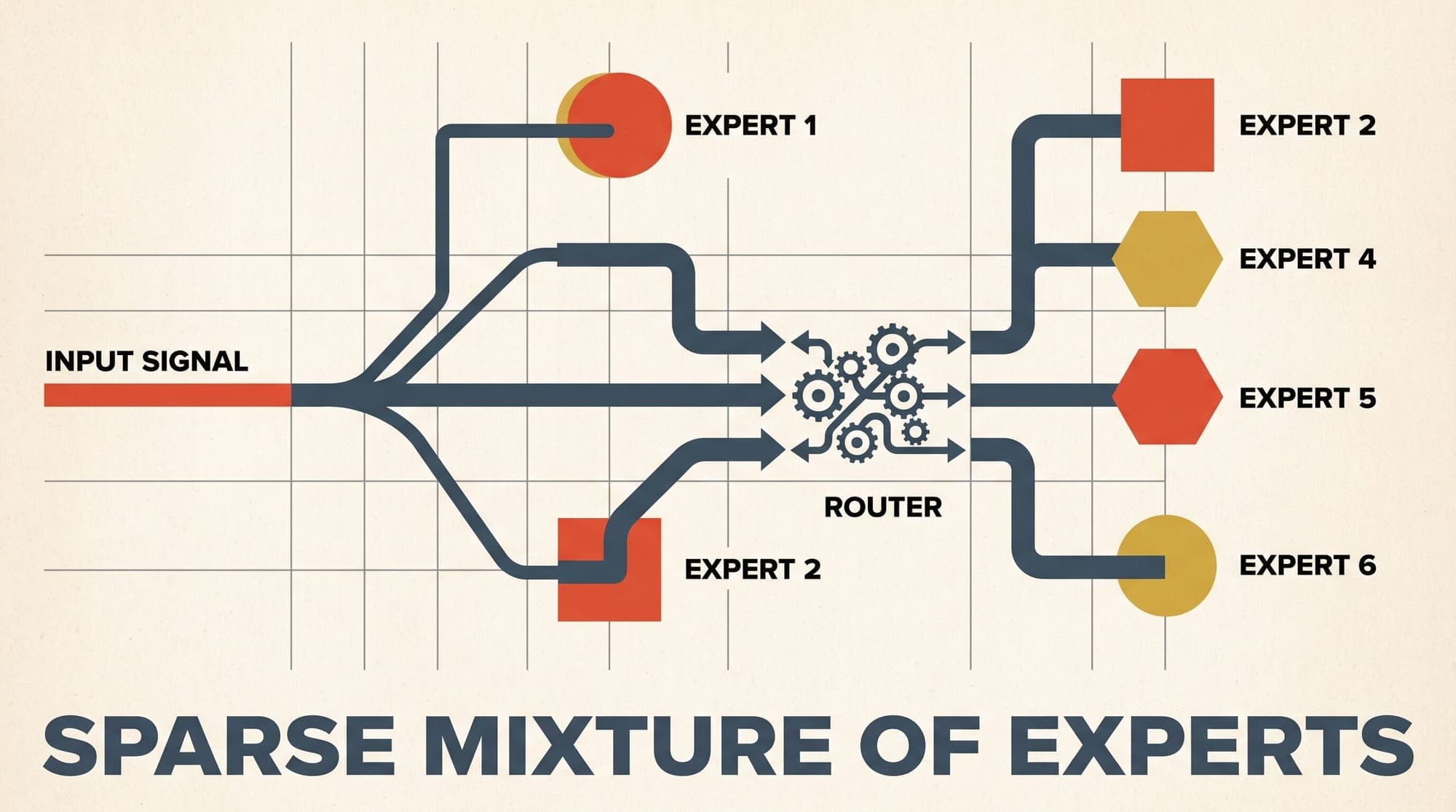
Scaling dense Transformer architectures encounters a fundamental computational constraint: increasing total parameter capacity quadratically expands training compute and linearly increases inference latency per token. Sparse Mixture of Experts (MoE) architectures decouple parameter count from per-token compute by replacing monolithic feed-forward network (FFN) blocks with an ensemble of specialized sub-networks, dynamically activating only a small subset of parameters per token.

First popularized in modern deep learning by Shazeer et al. (2017) and refined for massive scale by Fedus et al. (2021) in the Switch Transformer, MoE architectures underpin frontier systems such as Mixtral 8x7B, DBRX, Grok-1, and DeepSeek-V3. However, conditional execution introduces complex routing dynamics, representation collapse, and distributed hardware bottlenecks that require precise mathematical formulation and auxiliary regularization.

The Sparse MoE Formulation: Decoupling Compute from Capacity

In a standard dense Transformer layer, every input token $x \in \mathbb{R}^d$ passes through identical multi-head self-attention and feed-forward sub-layers. The dense FFN computes:

$$\text{FFN}(x) = W_2 \cdot \sigma(W_1 x + b_1) + b_2$$

where $W_1 \in \mathbb{R}^{d_{ffn} \times d}$, $W_2 \in \mathbb{R}^{d \times d_{ffn}}$, and $\sigma$ is a non-linear activation function such as GeLU or SwiGLU.

A Sparse MoE layer substitutes the singular FFN with a collection of $E$ independent expert networks $\{E_i\}_{i=1}^E$, coordinated by a parameterized router (gating network) $G(x)$. The layer output $y \in \mathbb{R}^d$ is the weighted linear combination of expert outputs:

$$y = \sum_{i=1}^E G(x)_i E_i(x)$$

where $G(x) \in \mathbb{R}^E$ is a sparse gating vector satisfying $\sum_{i=1}^E G(x)_i = 1$ and $G(x)_i \ge 0$. Sparsity requires that for any given token $x$, at most $k \ll E$ entries of $G(x)$ are non-zero. When $k=1$ or $k=2$, the computational FLOPs per token remain equivalent to a small dense model, while the parameter footprint scales with $E$.

+-------------------------------------------------------------------+
|                     Input Token Vector x in R^d                   |
+-------------------------------------------------------------------+
                                  |
         +------------------------+------------------------+
         |                                                 |
         v                                                 v
+-----------------+                               +-----------------+
|  Router G(x)    |                               |  Shared Expert  |
|  x * W_g        |                               |  E_shared(x)    |
+-----------------+                               +-----------------+
         |                                                 |
         | Top-k Dispatch (k of E)                         |
         +-------------+-------------+                     |
         |             |             |                     |
         v             v             v                     |
   +-----------+ +-----------+ +-----------+               |
   | Expert 1  | | Expert 2  | | Expert E  |               |
   | E_1(x)    | | E_2(x)    | | E_E(x)    |               |
   +-----------+ +-----------+ +-----------+               |
         |             |             |                     |
         +------+------+------+------+                     |
                |                                          |
                v                                          v
      Weighted Sum: Sum(G(x)_i * E_i(x))        +    E_shared(x)
                |                                          |
                +--------------------+---------------------+
                                     |
                                     v
                           Layer Output Vector y

Router Gating Topologies: From Noisy Top-k to Softmax Renormalization

The router function $G(x)$ maps continuous hidden states to discrete expert selections and continuous combination weights. Multiple routing formulations have evolved to balance computational efficiency and gradient propagation.

1. Noisy Top-k Gating

In Shazeer et al. (2017), gating decisions incorporate tunable Gaussian noise to promote exploratory routing during initial training stages:

$$H(x)_i = (x \cdot W_g)_i + \epsilon \cdot \text{Softplus}((x \cdot W_{noise})_i), \quad \epsilon \sim \mathcal{N}(0, 1)$$

where $W_g, W_{noise} \in \mathbb{R}^{d \times E}$. The top-$k$ elements are preserved while all other logits are masked to $-\infty$:

$$\text{KeepTopK}(v, k)_i = \begin{cases} v_i & \text{if } v_i \in \text{TopK}(v, k) \\ -\infty & \text{otherwise} \end{cases}$$

The sparse gating weights are computed via Softmax:

$$G(x) = \text{Softmax}(\text{KeepTopK}(H(x), k))$$

2. Deterministic Top-k with Softmax Renormalization

Modern large language models such as Mixtral 8x7B (Jiang et al., 2024) remove the noise parameterization during standard forward passes. The router computes unnormalized logits $h(x) = x W_g$, applies a Softmax over all $E$ experts, selects the top-$k$ indices $\mathcal{T} = \text{TopK}(h(x), k)$, and renormalizes the weights:

$$s_i(x) = \frac{e^{h(x)_i}}{\sum_{j=1}^E e^{h(x)_j}}$$

$$G(x)_i = \begin{cases} \frac{s_i(x)}{\sum_{j \in \mathcal{T}} s_j(x)} & \text{if } i \in \mathcal{T} \\ 0 & \text{otherwise} \end{cases}$$

Renormalization ensures that $\sum_{i \in \mathcal{T}} G(x)_i = 1$, preventing gradient attenuation when non-selected experts accumulate significant probability mass.

3. Single-Expert Routing (Switch Transformer)

The Switch Transformer (Fedus et al., 2021) sets $k=1$. Each token routes to exactly one expert:

$$i^* = \text{argmax}_i (x W_g)_i, \quad G(x)_{i^<em>} = s_{i^</em>}(x)$$

Top-1 routing reduces communication overhead during distributed expert parallelism, as each token requires a single point-to-point transfer rather than multi-cast fan-out.

Capacity Factors, Buffer Sizing, and Token Dropping

In distributed training and inference, tokens are partitioned across accelerator devices hosting different experts using all-to-all collective communications (all_to_all_single). Because static tensor shapes are required for efficient hardware execution and non-blocking CUDA kernels, each expert is allocated a fixed batch buffer size termed Expert Capacity ($E_C$).

Given a batch of $T$ tokens and $E$ experts, the expert capacity is defined by:

$$E_C = \left\lceil \frac{T \cdot k}{E} \times C \right\rceil$$

where $C \ge 1.0$ is the Capacity Factor.

• $C = 1.0$ (Exact Capacity): Allocates buffer space assuming perfectly uniform token distribution across all $E$ experts.
• $C > 1.0$ (Slack Capacity): Allocates additional buffer headroom (such as $C = 1.25$ or $C = 1.5$) to accommodate routing variance across batches.
• Token Dropping: If the router assigns $M_i > E_C$ tokens to expert $i$, the excess $M_i - E_C$ tokens cannot fit into the expert's static execution buffer. These dropped tokens bypass the expert layer entirely, passing through the residual connection unchanged:

$$y = x \quad (\text{for dropped tokens})$$

Token dropping degrades model perplexity if unmitigated. However, setting $C$ too high wastes accelerator memory and induces communication padding overhead for under-utilized experts.

Representation Collapse and the Differentiable Load Balancing Loss

A fundamental pathology in naive MoE training is expert collapse (winner-take-all routing). If a small subset of experts initially receives slightly more tokens, their parameter gradients update faster, improving their representation capacity relative to unselected experts. The router subsequently assigns even more tokens to these dominant experts, starving the remaining sub-networks and reducing the effective capacity to that of a dense model.

To enforce uniform expert utilization, MoE architectures optimize an auxiliary load balancing loss $\mathcal{L}_{aux}$ alongside the primary language modeling cross-entropy loss $\mathcal{L}_{LM}$.

Total Loss = L_LM(tokens) + alpha * L_aux(routing) + c_z * L_z(logits)

Mathematical Derivation of Switch Auxiliary Loss

Let $\mathcal{B}$ denote a batch of $T$ tokens. For each expert $i \in \{1, \dots, E\}$:

1. Fraction of Tokens Dispatched ($f_i$): The discrete empirical fraction of tokens routed to expert $i$:

$$f_i = \frac{1}{T} \sum_{x \in \mathcal{B}} \mathbb{I}(\text{argmax}_j (x W_g)_j = i)$$

1. Average Routing Probability ($P_i$): The continuous expected probability mass assigned to expert $i$ across the batch:

$$P_i = \frac{1}{T} \sum_{x \in \mathcal{B}} s_i(x) = \frac{1}{T} \sum_{x \in \mathcal{B}} \frac{e^{(x W_g)_i}}{\sum_{j=1}^E e^{(x W_g)_j}}$$

The auxiliary loss is defined as the scaled dot product between the dispatch vector $f$ and probability vector $P$:

$$\mathcal{L}_{aux} = \alpha \cdot E \sum_{i=1}^E f_i \cdot P_i$$

where $\alpha$ is a balancing coefficient (typically $\alpha \in [10^{-3}, 10^{-2}]$).

Why the $f_i \cdot P_i$ Formulation Works

The objective achieves its global minimum when token routing is uniformly distributed across all experts:

• By Cauchy-Schwarz and Jensen's inequality:

$$\sum_{i=1}^E f_i P_i \ge \frac{1}{E} \left( \sum_{i=1}^E f_i \right) \left( \sum_{i=1}^E P_i \right) = \frac{1}{E} (1)(1) = \frac{1}{E}$$

• At uniform balance ($f_i = \frac{1}{E}$ and $P_i = \frac{1}{E}$ for all $i$):

$$\mathcal{L}_{aux} = \alpha \cdot E \cdot \sum_{i=1}^E \left( \frac{1}{E} \cdot \frac{1}{E} \right) = \alpha \cdot E \cdot \frac{1}{E} = \alpha$$

• At complete collapse ($f_1 = 1, P_1 = 1$ and $f_{j>1} = 0, P_{j>1} = 0$):

$$\mathcal{L}_{aux} = \alpha \cdot E \cdot (1 \cdot 1) = \alpha E$$

Because $f_i$ is computed via discrete argmax, it is non-differentiable and treated as a constant during backpropagation. However, $P_i$ is smooth and differentiable with respect to the router weights $W_g$.

The gradient with respect to the router logit $h_i(x) = (x W_g)_i$ is:

$$\frac{\partial \mathcal{L}_{aux}}{\partial h_i(x)} = \frac{\alpha E}{T} \sum_{j=1}^E f_j \frac{\partial P_j}{\partial h_i(x)} = \frac{\alpha E}{T} \sum_{j=1}^E f_j \left( s_j(x) (\delta_{ij} - s_i(x)) \right) = \frac{\alpha E}{T} s_i(x) \left( f_i - \sum_{j=1}^E f_j s_j(x) \right)$$

When expert $i$ is overloaded ($f_i > \frac{1}{E}$), the gradient $\frac{\partial \mathcal{L}_{aux}}{\partial h_i(x)} > 0$, penalizing $W_g$ to decrease $h_i(x)$ for subsequent tokens. Conversely, underutilized experts receive negative gradient pressure, driving their selection probabilities upward.

Numerical Stability: The Router z-loss

During long pre-training runs with FP16 or BF16 mixed precision, router logits $h_i(x)$ tend to grow in magnitude. Large positive logits produce extreme values in $\sum_{j} e^{h_j(x)}$, triggering floating-point overflow and numerical instability in the Softmax backward pass.

To stabilize router optimization, Zoph et al. (2022) introduced the Router z-loss in ST-MoE:

$$\mathcal{L}_z = \frac{c_z}{T} \sum_{t=1}^T \left( \log \sum_{i=1}^E e^{h_i(x_t)} \right)^2$$

where $c_z$ is a regularization hyperparameter (typically $c_z = 10^{-4}$). The z-loss penalizes large values of the log partition function $\log Z = \log \sum e^{h_i}$, forcing router logits toward zero without constraining the relative differences between expert scores.

Structural Evolutions: Fine-Grained Segmentation and Shared Experts

Recent architectures move beyond standard Top-2 MoE routing by re-architecting the expert granularity and parameter partitioning.

Traditional MoE (8 Large Experts, Top-2):
Combinations = C(8, 2) = 28 expert combinations

DeepSeekMoE Fine-Grained (64 Small Sub-Experts, Top-8 + Shared):
Combinations = C(64, 8) = 4,426,165,368 combinations (Identical Active FLOPs)

Structural Comparison Across Paradigms

• Standard Top-k MoE (e.g., Mixtral 8x7B): 8 large experts per layer ($1.0 \times$ standard FFN), routing top-2 via renormalized softmax, combinatorial capacity $\binom{8}{2} = 28$ paths, capacity factor $C \in [1.25, 1.5]$, balanced via continuous-discrete auxiliary loss $\mathcal{L}_{aux}$.
• Switch Transformer: 64 to 2048 experts per layer ($1.0 \times$ standard FFN), routing top-1 via deterministic argmax, combinatorial capacity $\binom{E}{1} = E$ paths, capacity factor $C \in [1.0, 1.25]$, balanced via linear-scaling auxiliary loss $\mathcal{L}_{aux}$.
• Fine-Grained MoE with Shared Experts (DeepSeekMoE / DeepSeek-V3): 64 to 256 routed sub-experts ($\frac{1}{4} \times$ or $\frac{1}{8} \times$ standard FFN size) plus 1 to 2 unconditionally shared experts, routing top-6 to top-8 sub-experts, combinatorial capacity $\binom{64}{8} \approx 4.4 \times 10^9$ paths, dropless dynamic buffer routing, balanced via step-wise logit bias calibration ($h_i + b_i$) without auxiliary loss backpropagation.

1. Fine-Grained Expert Segmentation

Introduced in DeepSeekMoE (Dai et al., 2024), fine-grained segmentation divides each standard expert of intermediate dimension $d_{ffn}$ into $m$ smaller sub-experts of dimension $d_{ffn} / m$. Rather than selecting $k$ large experts out of $N$, the router selects $m \cdot k$ sub-experts out of $m \cdot N$.

This preserves identical computational FLOPs and parameter memory while expanding the combinatorial representation space from $\binom{N}{k}$ to $\binom{mN}{mk}$. Finer granularity enables more nuanced functional specialization across token domains.

2. Isolated Shared Experts

In standard MoE routing, common linguistic patterns, syntactic markers, and general task knowledge are redundantly learned across multiple specialized experts. DeepSeekMoE isolates $K_s$ shared experts that are unconditionally active for all tokens:

$$y = \sum_{j=1}^{K_s} E_{j}^{\text{shared}}(x) + \sum_{i \in \mathcal{T}_{routed}} G(x)_i E_i(x)$$

Shared experts capture invariant foundational representations, allowing the routed experts to focus exclusively on domain-specific features without parameter redundancy.

3. Auxiliary-Loss-Free Dynamic Bias Routing

In large-scale training runs, balancing auxiliary losses against the primary task loss introduces a gradient conflict: strong auxiliary loss forces uniform utilization at the expense of optimal task routing, while weak auxiliary loss allows expert collapse.

DeepSeek-V3 (DeepSeek-AI, 2024) eliminates $\mathcal{L}_{aux}$ from the backward gradient graph entirely. Instead, the router adds an explicit bias term $b_i$ to the routing logits:

$$h_i(x) = (x W_g)_i + b_i$$

The bias terms $b_i$ are dynamically adjusted at the end of each training step based on expert load:

$$b_i^{(t+1)} = b_i^{(t)} + \gamma \cdot \text{sign}\left( \frac{1}{E} - f_i^{(t)} \right)$$

where $\gamma$ is a step update hyperparameter. Because $b_i$ is updated outside the optimizer backward graph, the language model gradients remain uncorrupted by artificial balance objectives, maximizing cross-entropy optimization while maintaining balanced hardware utilization.

Sources

• Outrageously Large Neural Networks: The Sparsely-Gated Mixture-of-Experts Layer (Shazeer et al., 2017)
• Switch Transformers: Scaling to Trillion Parameter Models with Simple and Efficient Sparsity (Fedus et al., 2021)
• GShard: Scaling Giant Models with Conditional Computation and Automatic Sharding (Lepikhin et al., 2020)
• ST-MoE: Designing Stable and Transferable Sparse Expert Models (Zoph et al., 2022)
• Mixtral of Experts (Jiang et al., 2024)
• DeepSeekMoE: Towards Ultimate Expertise in Shared and Fine-Grained Routing (Dai et al., 2024)
• DeepSeek-V3 Technical Report (DeepSeek-AI, 2024)