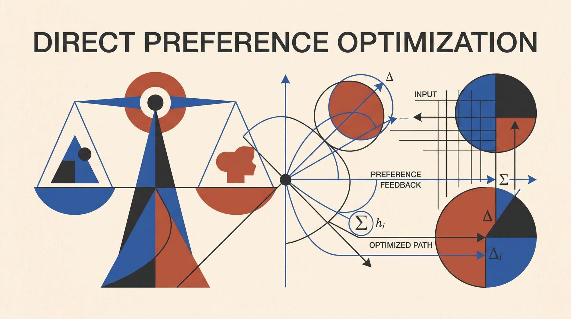
Direct Preference Optimization: How Implicit Reward Modeling Simplified LLM Alignment

Direct Preference Optimization (DPO) has emerged as a cornerstone of post-training alignment across modern open and proprietary language models, including Meta's Llama series, Mistral, and Qwen. While early alignment pipelines relied on complex reinforcement learning loops with separate reward models, DPO reformulates the preference optimization problem into a single, closed-form classification objective.

By demonstrating that a language model implicitly defines its own reward function, DPO eliminates the need for dynamic token generation, separate value networks, and reinforcement learning policy gradients during preference tuning.

The Classical RLHF Pipeline

Following supervised fine-tuning (SFT) on curated instruction demonstrations, raw language models often generate fluent but undesirable, unhelpful, or untruthful outputs. The classical framework for steering model behavior, Reinforcement Learning from Human Feedback (RLHF), was established in Ziegler et al. (2019) and Stiennon et al. (2020), and later popularized at scale by Ouyang et al. (2022) in InstructGPT.

The standard RLHF workflow operates in three distinct stages:

1. Supervised Fine-Tuning (SFT): Pre-trained base models are fine-tuned on high-quality instruction-response pairs to produce an initial policy, denoted as $\pi_{\text{SFT}}$ or $\pi_{\text{ref}}$.
2. Reward Model Training: Human annotators or automated judges evaluate pairs of model completions $(y_w, y_l)$ for a given prompt $x$, marking $y_w$ as the preferred (winning) completion and $y_l$ as the dispreferred (losing) completion. A separate reward model $r_\phi(x, y)$ is trained to score responses using the Bradley-Terry preference model from Bradley and Terry (1952):

$$P(y_w \succ y_l \mid x) = \sigma\left(r_\phi(x, y_w) - r_\phi(x, y_l)\right) = \frac{1}{1 + e^{-(r_\phi(x, y_w) - r_\phi(x, y_l))}}$$

The reward model parameters $\phi$ are optimized by minimizing the negative log-likelihood across the dataset $\mathcal{D}$:

$$\mathcal{L}_R(\phi) = -\mathbb{E}_{(x, y_w, y_l) \sim \mathcal{D}}\left[\log \sigma\left(r_\phi(x, y_w) - r_\phi(x, y_l)\right)\right]$$

1. Reinforcement Learning (PPO): The target policy $\pi_\theta$ is optimized against the static reward model $r_\phi$ using Proximal Policy Optimization (Schulman et al., 2017). To prevent the policy from degenerating into reward hacking or collapsing its language distribution, an explicit Kullback-Leibler (KL) divergence penalty against the reference model $\pi_{\text{ref}}$ is added to the objective:

$$\max_{\pi_\theta} \mathbb{E}_{x \sim \mathcal{D}, y \sim \pi_\theta(y \mid x)}\left[r_\phi(x, y) - \beta D_{\text{KL}}\left(\pi_\theta(y \mid x) \parallel \pi_{\text{ref}}(y \mid x)\right)\right]$$

Here, $\beta$ is a hyperparameter controlling the strength of the KL regularization penalty.

The Operational Bottlenecks of PPO

While effective, PPO-based RLHF introduces severe engineering overhead and mathematical instability during training:

• GPU Memory Footprint: PPO requires loading up to four distinct model instances into GPU clusters simultaneously: the active actor policy $\pi_\theta$, the frozen reference policy $\pi_{\text{ref}}$, the reward model $r_\phi$, and the critic/value network $V_\psi$ used for generalized advantage estimation.
• Inference Rollout Latency: Reinforcement learning is an online procedure requiring constant auto-regressive generation. During each training step, the actor model must sample new completions $y \sim \pi_\theta(y \mid x)$ across the batch, feed them to the reward model and value network, and compute step-by-step token rewards. These dynamic rollouts make training memory-bound and computationally slow compared to standard gradient backpropagation.
• Training Instability: Actor-critic reinforcement learning methods are sensitive to learning rates, value function initialization, advantage clipping thresholds, and reward scaling drift. If the value function fails to converge accurately, gradient updates destabilize the policy.

The Mathematical Core of Direct Preference Optimization

Introduced by Rafael Rafailov, Archit Sharma, Eric Mitchell, Stefano Ermon, Christopher D. Manning, and Chelsea Finn in Direct Preference Optimization: Your Language Model is Secretly a Reward Model (NeurIPS 2023), DPO bypasses explicit reward modeling and PPO altogether.

1. The Closed-Form Optimal Policy

Under the standard KL-regularized reward maximization objective:

$$\max_{\pi} \mathbb{E}_{x \sim \mathcal{D}, y \sim \pi(y \mid x)}\left[r(x, y)\right] - \beta D_{\text{KL}}\left(\pi(y \mid x) \parallel \pi_{\text{ref}}(y \mid x)\right)$$

The exact analytical solution for the optimal policy $\pi^*(y \mid x)$ can be derived using calculus of variations and the properties of Gibbs distributions:

$$\pi^*(y \mid x) = \frac{1}{Z(x)} \pi_{\text{ref}}(y \mid x) \exp\left(\frac{1}{\beta} r(x, y)\right)$$

where $Z(x) = \sum_y \pi_{\text{ref}}(y \mid x) \exp\left(\frac{1}{\beta} r(x, y)\right)$ is the partition function normalizing the distribution over all possible completions.

2. Reparameterizing the Reward

By taking the natural logarithm of both sides and rearranging terms, the ground-truth reward $r(x, y)$ can be expressed strictly as a function of the optimal policy $\pi^*$, the reference policy $\pi_{\text{ref}}$, and the partition function:

$$r(x, y) = \beta \log \frac{\pi^*(y \mid x)}{\pi_{\text{ref}}(y \mid x)} + \beta \log Z(x)$$

This relationship reveals that any parameterized language model policy $\pi_\theta$ implicitly defines a reward function:

$$r_\theta(x, y) = \beta \log \frac{\pi_\theta(y \mid x)}{\pi_{\text{ref}}(y \mid x)} + \beta \log Z(x)$$

3. Deriving the DPO Loss Function

When substituting this implicit reward formulation into the Bradley-Terry preference probability, the prompt-dependent partition function $Z(x)$ cancels out entirely:

$$r_\theta(x, y_w) - r_\theta(x, y_l) = \beta \left(\log \frac{\pi_\theta(y_w \mid x)}{\pi_{\text{ref}}(y_w \mid x)} + \log Z(x)\right) - \beta \left(\log \frac{\pi_\theta(y_l \mid x)}{\pi_{\text{ref}}(y_l \mid x)} + \log Z(x)\right)$$

$$r_\theta(x, y_w) - r_\theta(x, y_l) = \beta \log \frac{\pi_\theta(y_w \mid x)}{\pi_{\text{ref}}(y_w \mid x)} - \beta \log \frac{\pi_\theta(y_l \mid x)}{\pi_{\text{ref}}(y_l \mid x)}$$

The probability that preference data prefers $y_w$ over $y_l$ becomes:

$$P(y_w \succ y_l \mid x) = \sigma\left(\beta \log \frac{\pi_\theta(y_w \mid x)}{\pi_{\text{ref}}(y_w \mid x)} - \beta \log \frac{\pi_\theta(y_l \mid x)}{\pi_{\text{ref}}(y_l \mid x)}\right)$$

By applying maximum likelihood estimation directly to the preference dataset $\mathcal{D} = \{(x, y_w, y_l)\}$, the final DPO training loss is formulated as:

$$\mathcal{L}_{\text{DPO}}(\theta; \pi_{\text{ref}}) = -\mathbb{E}_{(x, y_w, y_l) \sim \mathcal{D}}\left[\log \sigma\left(\beta \log \frac{\pi_\theta(y_w \mid x)}{\pi_{\text{ref}}(y_w \mid x)} - \beta \log \frac{\pi_\theta(y_l \mid x)}{\pi_{\text{ref}}(y_l \mid x)}\right)\right]$$

Gradient Dynamics and Implicit Weighting

Analyzing the gradient of the DPO loss with respect to the model parameters $\theta$ explains how updates behave during training:

$$\nabla_\theta \mathcal{L}_{\text{DPO}}(\theta) = -\beta \mathbb{E}_{(x, y_w, y_l)}\left[\sigma\left(\hat{r}_\theta(x, y_l) - \hat{r}_\theta(x, y_w)\right) \left(\nabla_\theta \log \pi_\theta(y_w \mid x) - \nabla_\theta \log \pi_\theta(y_l \mid x)\right)\right]$$

where $\hat{r}_\theta(x, y) = \beta \log \frac{\pi_\theta(y \mid x)}{\pi_{\text{ref}}(y \mid x)}$ represents the implicit reward assigned by the policy.

The gradient structure consists of two intuitive components:

1. Directional Push-Pull: The vector term $(\nabla_\theta \log \pi_\theta(y_w \mid x) - \nabla_\theta \log \pi_\theta(y_l \mid x))$ directly increases the likelihood of preferred completions $y_w$ while decreasing the likelihood of dispreferred completions $y_l$.
2. Error-Weighted Scalar Coefficient: The scaling factor $\sigma\left(\hat{r}_\theta(x, y_l) - \hat{r}_\theta(x, y_w)\right)$ measures how poorly the model currently ranks the pair. If the model already assigns a much higher implicit reward to $y_w$ than $y_l$, the coefficient approaches zero and produces minimal gradient updates. Conversely, when the model incorrectly favors the losing completion ($r_\theta(x, y_l) > r_\theta(x, y_w)$), the gradient scale increases, forcing aggressive parameter correction.

Practical Advantages in Production

The transition from PPO to DPO delivers several tangible benefits for model development:

• Simplified Architecture: Training requires only the target policy $\pi_\theta$ and a frozen forward pass through $\pi_{\text{ref}}$. Critic networks and standalone reward models are eliminated.
• Offline Supervised Stability: DPO runs as a standard supervised classification loss on static preference pairs. It avoids the hyperparameter sensitivity, advantage estimation variance, and rollout divergence common to RL.
• Compute Efficiency: Without the requirement to generate new token completions during the training step, DPO matches standard fine-tuning throughput, scaling linearly with batch size and context length.

Limitations and Subsequent Extensions

Despite its strengths, standard DPO exhibits known structural failure modes that have driven subsequent research:

1. Verbosity and Length Bias

Because DPO optimizes cumulative sequence log-probabilities, longer outputs can accumulate higher implicit reward deltas. Models fine-tuned with unconstrained DPO often develop an artificial verbosity bias, generating unnecessarily long answers to maximize token-level likelihood sums. Researchers address this with length-normalized formulations and data deduplication.

2. Out-of-Distribution Degradation

When trained over multiple epochs, standard DPO can decrease the probability of dispreferred responses to near-zero ($-\infty$ in log-space), leading to over-optimization and degradation on tasks outside the preference distribution. Azar et al. (2023) introduced Identity Preference Optimization (IPO), adding a quadratic regularization term to prevent policy over-confidence:

$$\mathcal{L}_{\text{IPO}}(\theta) = \mathbb{E}_{(x, y_w, y_l)}\left[\left(\log \frac{\pi_\theta(y_w \mid x)}{\pi_{\text{ref}}(y_w \mid x)} - \log \frac{\pi_\theta(y_l \mid x)}{\pi_{\text{ref}}(y_l \mid x)} - \frac{1}{2\tau}\right)^2\right]$$

3. Unpaired Feedback (KTO)

Standard DPO requires strictly paired comparisons $(y_w, y_l)$ for every prompt. In Ethayarajh et al. (2024), the authors introduced Kahneman-Tversky Optimization (KTO), which applies prospect theory to optimize models on unpaired binary signals (upvotes/downvotes) without needing pairwise comparisons.

4. Online and Iterative DPO

Offline DPO trains strictly on historical dataset distributions. When the active policy $\pi_\theta$ drifts away from the data distribution of the static dataset, performance gains plateau. Modern post-training pipelines often adopt Iterative or Online DPO, where the current model generates new candidate responses, an automated judge ranks them, and DPO is applied over successive generations.

Sources

• Direct Preference Optimization: Your Language Model is Secretly a Reward Model (Rafailov et al., 2023)
• Training language models to follow instructions with human feedback (Ouyang et al., 2022)
• Fine-Tuning Language Models from Human Preferences (Ziegler et al., 2019)
• A General Theoretical Paradigm to Understand Learning from Human Preferences (Azar et al., 2023)
• KTO: Model Alignment as Prospect Theoretic Optimization (Ethayarajh et al., 2024)
• Proximal Policy Optimization Algorithms (Schulman et al., 2017)
• Rank Analysis of Incomplete Block Designs: I. The Method of Paired Comparisons (Bradley & Terry, 1952)