Vector Quantization and VQ-VAEs: How Discrete Codebooks, Straight-Through Estimators, and Commitment Losses Power Multimodal Tokenization

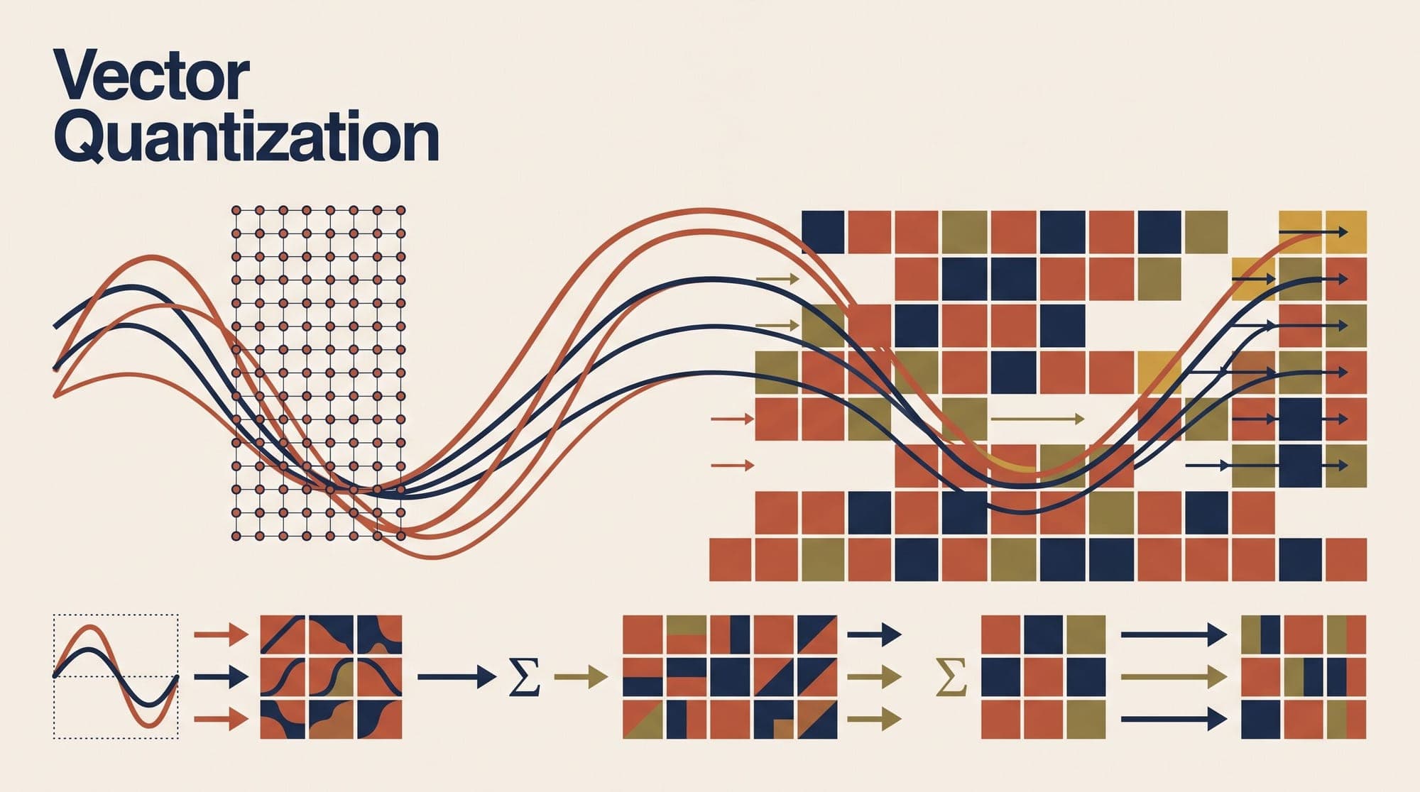
Autoregressive sequence models excel at discrete token prediction. In natural language processing, words and subwords map onto categorical vocabularies where token identity is exact and cross-entropy loss provides direct likelihood optimization. Continuous multi-dimensional signals—such as images, video frames, raw audio waveforms, and robotic sensorimotor trajectories—present a fundamental mismatch for standard transformer architectures.

Historically, variational autoencoders (VAEs) bridged raw continuous data and latent representations by mapping inputs to parameterized Gaussian distributions. However, standard continuous VAEs suffer from posterior collapse: when paired with powerful autoregressive decoders, the decoder often ignores the continuous latent variable entirely, as the Kullback-Leibler (KL) divergence penalty forces the posterior to match an uninformative standard normal prior.

Vector Quantized Variational Autoencoders (VQ-VAEs) resolved this bottleneck by replacing continuous latent spaces with a discrete, learnable codebook. By framing continuous representation learning as deterministic nearest-neighbor vector quantization and employing a straight-through estimator to bypass non-differentiable step functions, VQ-VAEs provide the discrete tokenization backbone that powers modern multimodal foundation models, autoregressive image generators, and neural audio codecs.

The Mathematical Framework of Vector Quantization

A standard VQ-VAE pipeline consists of three core components: an encoder network $E$, a discrete codebook (dictionary) $\mathcal{E}$, and a decoder network $G$.

Given an input $x$ (such as an image of dimension $H \times W \times C$), the encoder produces a continuous latent feature map:

$$z_e(x) = E(x) \in \mathbb{R}^{h \times w \times D}$$

Here, $h \times w$ represents the spatially downsampled resolution (for example, an $8\times$ or $16\times$ compression factor), and $D$ denotes the feature channel dimensionality.

The codebook $\mathcal{E}$ is defined as a finite set of $K$ learnable embedding vectors in the same $D$-dimensional space:

$$\mathcal{E} = \{e_1, e_2, \dots, e_K\}, \quad e_k \in \mathbb{R}^D$$

For every spatial location $(i, j)$ in the continuous latent grid $z_e(x)$, the vector quantization operator $q(\cdot)$ replaces the continuous vector $z_e(x)_{i,j}$ with its closest counterpart in the codebook using Euclidean distance:

$$z_q(x)_{i,j} = e_k \quad \text{where} \quad k = \arg\min_{j \in \{1, \dots, K\}} \|z_e(x)_{i,j} - e_j\|_2$$

The spatial grid of continuous vectors is thus compressed into a 2D grid of discrete indices:

$$k_{i,j} \in \{1, 2, \dots, K\}$$

The quantized representation $z_q(x) \in \mathbb{R}^{h \times w \times D}$ is subsequently passed to the decoder $G$ to reconstruct the original input:

$$\hat{x} = G(z_q(x))$$

Because the latent space is completely discrete, the prior over latents is not assumed to be a static Gaussian. Instead, during downstream generative modeling, an expressive autoregressive model or masked transformer can be trained directly over the categorical index sequence without experiencing posterior collapse.

Bypassing the Gradient Bottleneck: Straight-Through Estimators

The nearest-neighbor argmin mapping is a step function whose derivative is zero almost everywhere and undefined at boundary transitions. Standard gradient backpropagation from the reconstruction loss through the quantized latent $z_q(x)$ to the encoder $z_e(x)$ is mathematically zero:

$$\frac{\partial z_q}{\partial z_e} = 0$$

To train the encoder end-to-end, VQ-VAE relies on the Straight-Through Estimator (STE) heuristic. During the forward pass, the quantized vector $z_q(x)$ is fed into the decoder. During the backward pass, the gradient of the loss with respect to $z_q(x)$ is copied directly to $z_e(x)$ without modification.

In computational graph implementations, this is expressed using the stop-gradient operator $\text{sg}[\cdot]$:

$$z_q = z_e + \text{sg}[z_q - z_e]$$

In the forward pass, $(z_e - z_e)$ cancels out, evaluating to $z_q$. In the backward pass, because $\text{sg}[z_q - z_e]$ has zero gradient, the derivative with respect to $z_e$ is simply the identity operator:

$$\nabla_{z_e} \mathcal{L} \approx \nabla_{z_q} \mathcal{L}$$

This allows reconstruction gradients from the decoder to flow directly back into the encoder parameters, adjusting encoder representations toward configurations that minimize reconstruction error.

The Tripartite Objective Function

Because the straight-through estimator copies gradients directly from $z_q$ to $z_e$, the codebook embeddings $e_k$ receive no gradients from the reconstruction loss. Furthermore, the encoder outputs $z_e(x)$ could theoretically grow arbitrarily large without committing to any codebook vector.

To resolve both dynamics, VQ-VAE introduces a composite loss function comprising three distinct terms:

$$\mathcal{L} = \mathcal{L}_{\text{recon}}(x, G(z_q)) + \|\text{sg}[z_e(x)] - z_q\|_2^2 + \beta \|z_e(x) - \text{sg}[z_q]\|_2^2$$

1. Reconstruction Loss

The first term, $\mathcal{L}_{\text{recon}}$, measures how accurately the decoder reconstructs the input from the discrete quantized representation. In the original VQ-VAE, this was implemented as mean squared error (MSE) or negative log-likelihood. In modern perceptual frameworks like VQGAN, this term is augmented with Learned Perceptual Image Patch Similarity (LPIPS) and patch-based adversarial Discriminator losses ($\mathcal{L}_{\text{adv}}$) to preserve sharp high-frequency textures.

2. Codebook Vector Quantization Loss

The second term, $\|\text{sg}[z_e(x)] - z_q\|_2^2$, optimizes the codebook vectors. By applying the stop-gradient operator to the encoder output $z_e(x)$, this term acts as dictionary learning (similar to K-means clustering), pulling the selected codebook vector $e_k$ closer to the encoder outputs mapped to that index.

3. Commitment Loss

The third term, $\beta \|z_e(x) - \text{sg}[z_q]\|_2^2$, prevents the encoder representations from fluctuating wildly. The stop-gradient on $z_q$ ensures that codebook vectors remain static with respect to this term, while the encoder is penalized if its output $z_e(x)$ drifts far from its chosen codeword. The scaling hyperparameter $\beta$ controls the strength of this commitment penalty, typically calibrated to $\beta = 0.25$.

Exponential Moving Average Updates

As an alternative to optimizing codebook embeddings via gradient descent on the vector quantization loss, empirical implementations frequently utilize Exponential Moving Average (EMA) updates. For each codebook entry $i$, the model tracks the count of assigned encoder vectors $N_i$ and the sum of assigned vectors $m_i$:

$$N_i^{(t)} := \gamma N_i^{(t-1)} + (1 - \gamma) n_i^{(t)}$$

$$m_i^{(t)} := \gamma m_i^{(t-1)} + (1 - \gamma) \sum_{j: q(z_j)=i} z_j^{(t)}$$

$$e_i^{(t)} := \frac{m_i^{(t)}}{N_i^{(t)}}$$

where $\gamma \in [0.9, 0.99]$ is a decay factor. EMA updates decouple dictionary updates from optimizer momentum states and learning rate schedules, yielding more stable codebook convergence.

Codebook Pathologies and Modern Mitigations

Despite their conceptual elegance, standard VQ-VAEs encounter several critical failure modes in practice.

Codebook Collapse and Dead Codewords

A pervasive issue in vector quantization is codebook underutilization (or codebook collapse). Early in training, if a subset of codewords is initialized slightly farther from the data distribution, they are never selected as nearest neighbors. Because unselected codewords receive neither gradient updates nor EMA counts, they remain inactive permanently. In severe cases, a codebook with $K = 8192$ vectors may utilize fewer than 200 active entries.

Common remedies include:

• Periodic K-Means Restarts: Inactive codewords with usage frequency below a predefined threshold are periodically re-initialized by sampling random continuous encoder vectors from the current training batch.
• L2 Normalized Quantization: Both the continuous encoder outputs $z_e$ and the codebook embeddings $e_k$ are projected onto the unit sphere ($\|z_e\|_2 = 1, \|e_k\|_2 = 1$). This restricts the search space to cosine similarity on a hypersphere, preventing vector magnitude drift from isolating codewords.

Residual Vector Quantization (RVQ)

To represent high-bandwidth signals such as 44.1kHz audio without requiring an intractable codebook size $K$, Residual Vector Quantization (RVQ) introduces a cascade of $N_q$ quantization stages:

$$z_{q, 1} = \text{quantize}(z, \mathcal{E}_1)$$

$$r_1 = z - z_{q, 1}$$

$$z_{q, 2} = \text{quantize}(r_1, \mathcal{E}_2)$$

$$z_q = \sum_{m=1}^{N_q} z_{q, m}$$

Each successive codebook quantizes the residual quantization error of the previous stage. Used in neural audio architectures such as SoundStream and EnCodec, RVQ achieves high bitrate fidelity while maintaining compact individual codebooks (such as 8 codebooks of size 1024 rather than one astronomical codebook of size $1024^8$).

Finite Scalar Quantization (FSQ)

To eliminate the engineering overhead of codebook optimization, commitment losses, and dead-codeword restarts entirely, Finite Scalar Quantization (FSQ) replaces vector lookup tables with independent scalar rounding.

FSQ projects the continuous latent representation to a very low dimensionality $d$ (typically $d \le 8$) and bounds each dimension to a fixed set of $L_i$ discrete integer levels:

$$\hat{z}_i = \text{round}\left( \left\lfloor \frac{L_i}{2} \right\rfloor \tanh(z_i) \right)$$

For example, choosing levels $[8, 5, 5, 5]$ yields an implicit codebook of size $8 \times 5 \times 5 \times 5 = 1000$ discrete tokens. FSQ achieves 100% codebook utilization by construction, requires zero auxiliary codebook or commitment losses, and relies solely on the standard straight-through estimator for backpropagation.

The Two-Stage Paradigm in Foundation Models

Vector quantization established the two-stage generation framework that underpins modern multimodal AI:

1. Stage 1 (Perceptual Compression): A convolutional or vision-transformer VQ-VAE / VQGAN is trained purely as an autoencoder to compress high-dimensional raw data into a grid of discrete tokens while minimizing reconstruction and perceptual loss.
2. Stage 2 (Autoregressive Prior Modeling): A generative transformer (such as a causal decoder or masked sequence model) is trained to predict the categorical token distribution over the discrete latent grid conditioned on text prompts, class labels, or previous sequence tokens.

By discretizing continuous perceptual modalities into vocabulary indices identical in structure to text tokens, vector quantization enables unified multimodal models to process text, images, and audio within a single transformer backbone.

Sources

• van den Oord, A., Vinyals, O., & Kavukcuoglu, K. (2017). Neural Discrete Representation Learning. Advances in Neural Information Processing Systems (NeurIPS 2017).
• Esser, P., Rombach, R., & Ommer, B. (2021). Taming Transformers for High-Resolution Image Synthesis. IEEE/CVF Conference on Computer Vision and Pattern Recognition (CVPR 2021).
• Mentzer, F., Minnen, D., Agustsson, E., & Tschannen, M. (2023). Finite Scalar Quantization: VQ-VAE Made Simple. arXiv preprint arXiv:2309.15505.
• Défossez, A., Copet, J., Synnaeve, G., & Adi, Y. (2022). High Fidelity Neural Audio Compression. arXiv preprint arXiv:2210.13438.
• Zeghidour, N., Luebs, A., Omran, A., Skoglund, J., & Tagliasacchi, M. (2021). SoundStream: An End-to-End Neural Audio Codec. IEEE/ACM Transactions on Audio, Speech, and Language Processing.
• Bengio, Y., Léonard, N., & Courville, A. (2013). Estimating or Propagating Gradients Through Stochastic Neurons for Conditional Computation. arXiv preprint arXiv:1308.3432.