Trust Region Policy Optimization: Mathematical Foundations, Monotonic Improvement Guarantees, and Conjugate Gradient Updates

In policy gradient reinforcement learning, optimization dynamics differ fundamentally from standard supervised learning. In supervised regression or classification, the underlying data distribution $P(x, y)$ remains stationary throughout training; a sub-optimal parameter update merely yields high loss on the current batch without corrupting future sample collection. In reinforcement learning, however, the parameter vector $\theta$ of a policy $\pi_\theta(a|s)$ defines both the action distribution and the state visitation distribution $\rho_\pi(s)$. A single excessive gradient step can push the policy into an unrecoverable region of parameter space, degrading performance and generating trajectories from which meaningful reward signals cannot be collected.

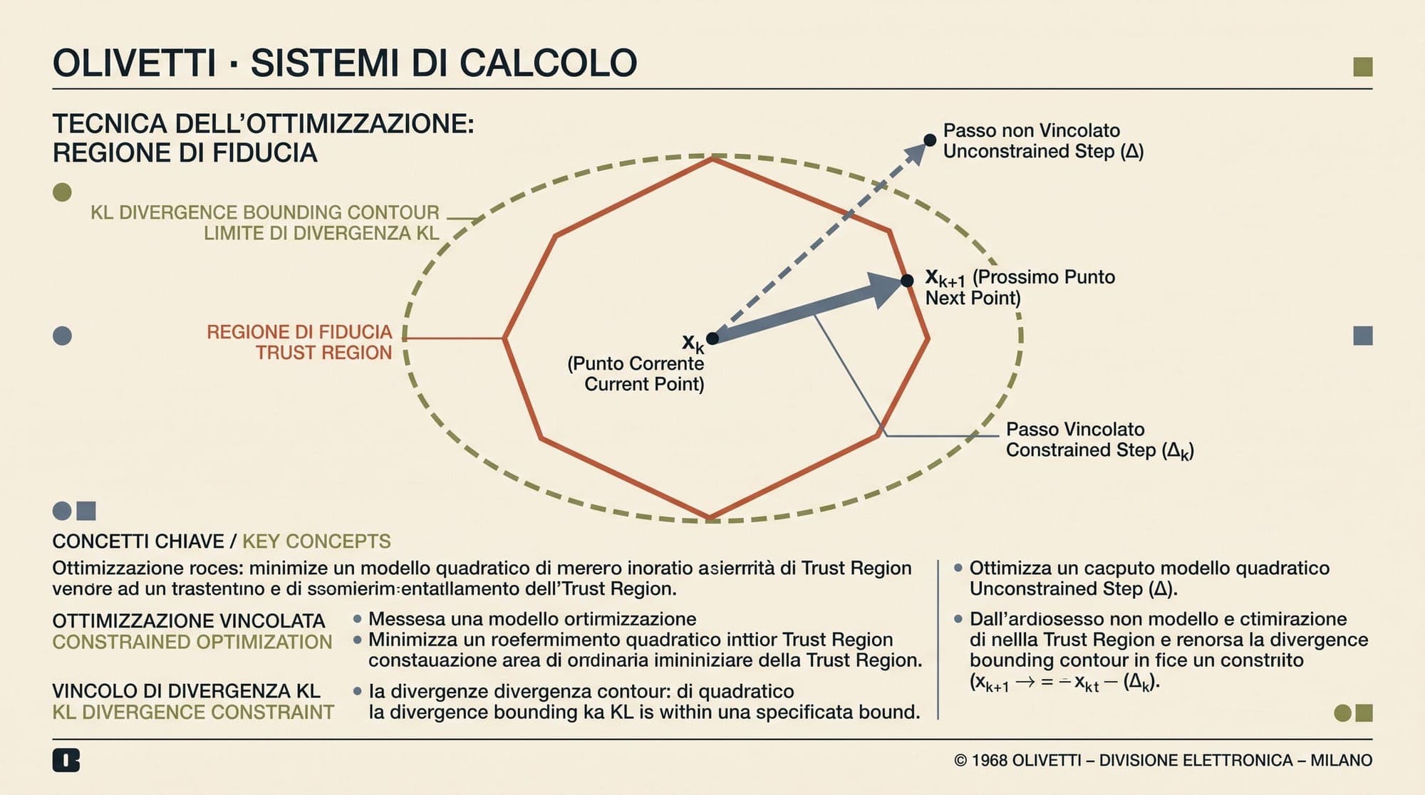
To resolve this instability, Schulman et al. (2015) introduced Trust Region Policy Optimization (TRPO). Building upon the theoretical foundations of Conservative Policy Iteration by Kakade and Langford (2002), TRPO proves that enforcing a statistical constraint on policy divergence guarantees monotonic policy improvement. By optimizing a local surrogate objective subject to an average Kullback-Leibler (KL) divergence constraint, and solving the resulting quadratic subproblem via the conjugate gradient method and automatic differentiation vector products, TRPO established the modern paradigm of constrained policy optimization.

The Policy Gradient Step-Size Dilemma

Standard policy gradient methods, derived from the Policy Gradient Theorem (Sutton et al., 1999), optimize the expected cumulative discounted return:

$$\eta(\pi) = \mathbb{E}_{\tau \sim \pi} \left[ \sum_{t=0}^\infty \gamma^t r(s_t, a_t) \right]$$

The analytical gradient of $\eta(\pi_\theta)$ with respect to parameter vector $\theta$ is given by:

$$\nabla_\theta \eta(\pi_\theta) = \mathbb{E}_{s \sim \rho_{\pi_\theta}, a \sim \pi_\theta} \left[ \nabla_\theta \log \pi_\theta(a|s) Q^{\pi_\theta}(s, a) \right]$$

In empirical implementations, parameters are updated via first-order gradient ascent:

$$\theta_{k+1} = \theta_k + \alpha \nabla_\theta \eta(\pi_\theta)$$

This first-order formulation suffers from three severe mathematical and practical limitations:

1. Euclidean Geometry vs. Probability Manifolds: First-order gradient ascent measures step size $\alpha$ in parameter space Euclidean distance $\|\Delta \theta\|_2$. However, neural network parameterizations are highly non-linear; an identical Euclidean step $\|\Delta \theta\|_2 = \epsilon$ can cause a negligible change in policy distributions in flat regions of the parameter landscape, yet cause catastrophic shifts in steep regions.
2. State Distribution Shift: Evaluating the gradient under trajectories sampled from $\pi_{\theta_k}$ assumes that the current state visitation distribution $\rho_{\pi_{\theta_k}}$ remains valid for the updated policy $\pi_{\theta_{k+1}}$. If the step size is too large, the state visitation distribution shifts abruptly, invalidating prior value estimates.
3. Irreversible Performance Collapse: In supervised learning, bad updates can be corrected by subsequent mini-batches. In reinforcement learning, a policy that degrades produces degenerate trajectories (such as getting stuck in dead-end states), eliminating exploratory actions and preventing the policy from recovering.

Kakade and Langford's Relative Performance Identity

To formalize how an updated policy $\tilde{\pi}$ performs relative to an existing policy $\pi$, Kakade and Langford (2002) derived the exact relative performance identity:

$$\eta(\tilde{\pi}) = \eta(\pi) + \sum_s \rho_{\tilde{\pi}}(s) \sum_a \tilde{\pi}(a|s) A_\pi(s, a)$$

where $A_\pi(s, a) = Q_\pi(s, a) - V_\pi(s)$ is the advantage function under policy $\pi$, and $\rho_\pi(s) = \sum_{t=0}^\infty \gamma^t P(s_t = s | \pi)$ is the unnormalized discounted state visitation frequency.

This identity reveals that if $\sum_a \tilde{\pi}(a|s) A_\pi(s, a) \ge 0$ for all states $s$, then $\eta(\tilde{\pi}) \ge \eta(\pi)$, guaranteeing policy improvement. However, computing the expectation over $\rho_{\tilde{\pi}}(s)$ is intractable in practice because sampling trajectories from the un-evaluated candidate policy $\tilde{\pi}$ prior to optimization is impossible.

The Local Surrogate Objective

To make optimization tractable, Schulman et al. replace the unknown state distribution $\rho_{\tilde{\pi}}(s)$ with the known state distribution $\rho_\pi(s)$, defining the local surrogate objective $L_\pi(\tilde{\pi})$:

$$L_\pi(\tilde{\pi}) = \eta(\pi) + \sum_s \rho_\pi(s) \sum_a \tilde{\pi}(a|s) A_\pi(s, a)$$

For parameterized policies $\pi_\theta$, $L_{\theta_0}(\theta)$ matches the true objective $\eta(\pi_\theta)$ to first order at $\theta = \theta_0$:

$$L_{\theta_0}(\theta_0) = \eta(\pi_{\theta_0})$$

$$\left. \nabla_\theta L_{\theta_0}(\theta) \right|_{\theta = \theta_0} = \left. \nabla_\theta \eta(\pi_\theta) \right|_{\theta = \theta_0}$$

Consequently, a sufficiently small step that improves $L_{\theta_0}(\theta)$ is guaranteed to improve $\eta(\pi_\theta)$.

The Monotonic Improvement Bound

To establish how large a step can be taken before the approximation error between $L_\pi(\tilde{\pi})$ and $\eta(\tilde{\pi})$ overwhelms the improvement, Schulman et al. established the formal bound:

$$\eta(\tilde{\pi}) \ge L_\pi(\tilde{\pi}) - C \cdot D_{\text{KL}}^{\max}(\pi, \tilde{\pi})$$

where:

• $D_{\text{KL}}^{\max}(\pi, \tilde{\pi}) = \max_s D_{\text{KL}}(\pi(\cdot|s) \parallel \tilde{\pi}(\cdot|s))$
• $C = \frac{4 \epsilon \gamma}{(1 - \gamma)^2}$
• $\epsilon = \max_{s, a} |A_\pi(s, a)|$

This inequality serves as a Minorize-Maximization (MM) algorithm: by iteratively maximizing the right-hand side lower bound, the true objective $\eta(\pi)$ is guaranteed to improve monotonically at every step:

$$\eta(\pi_{k+1}) \ge M_k(\pi_{k+1}) \ge M_k(\pi_k) = \eta(\pi_k)$$

where $M_k(\pi) = L_{\pi_k}(\pi) - C \cdot D_{\text{KL}}^{\max}(\pi_k, \pi)$.

From Theoretical Penalties to Practical Trust Regions

While the theoretical bound guarantees monotonic improvement, the constant $C = \frac{4 \epsilon \gamma}{(1 - \gamma)^2}$ is extremely large in practical reinforcement learning tasks (where discount factor $\gamma \approx 0.99$, making $(1 - \gamma)^2 = 0.0001$). An unconstrained optimization of $L_\pi(\tilde{\pi}) - C \cdot D_{\text{KL}}^{\max}(\pi, \tilde{\pi})$ forces step sizes to be vanishingly small, stalling training progress.

Furthermore, evaluating the maximum KL divergence $D_{\text{KL}}^{\max}(\pi, \tilde{\pi})$ across the entire state space is computationally impossible in continuous or high-dimensional environments.

TRPO makes two critical transitions to turn this theoretical framework into a practical algorithm:

1. Average KL Divergence: Replace the maximum KL divergence with the expected KL divergence under the state visitation distribution $\rho_{\theta_{\text{old}}}$:

$$\bar{D}_{\text{KL}}(\theta_{\text{old}}, \theta) = \mathbb{E}_{s \sim \rho_{\theta_{\text{old}}}} \left[ D_{\text{KL}}(\pi_{\theta_{\text{old}}}(\cdot|s) \parallel \pi_\theta(\cdot|s)) \right]$$

1. Hard Trust Region Constraint: Instead of a penalty formulation with fixed coefficient $C$, cast optimization as a constrained maximization problem with a bounded trust region step size $\delta$:

$$\max_\theta L_{\theta_{\text{old}}}(\theta) \quad \text{subject to} \quad \bar{D}_{\text{KL}}(\theta_{\text{old}}, \theta) \le \delta$$

Using importance sampling, the surrogate objective $L_{\theta_{\text{old}}}(\theta)$ is rewritten in sample form:

$$L_{\theta_{\text{old}}}(\theta) = \mathbb{E}_{s \sim \rho_{\theta_{\text{old}}}, a \sim \pi_{\theta_{\text{old}}}} \left[ \frac{\pi_\theta(a|s)}{\pi_{\theta_{\text{old}}}(a|s)} A_{\theta_{\text{old}}}(s, a) \right]$$

Quadratic Approximation and the Natural Policy Gradient

To solve the constrained optimization problem numerically, TRPO applies a second-order Taylor series expansion around $\theta_{\text{old}}$:

1. Linear approximation of the objective:

$$L_{\theta_{\text{old}}}(\theta) \approx L_{\theta_{\text{old}}}(\theta_{\text{old}}) + g^T (\theta - \theta_{\text{old}})$$

where $g = \left. \nabla_\theta L_{\theta_{\text{old}}}(\theta) \right|_{\theta = \theta_{\text{old}}} = \mathbb{E} \left[ \nabla_\theta \log \pi_\theta(a|s) A(s, a) \right]$.

1. Quadratic approximation of the KL divergence constraint:

$$\bar{D}_{\text{KL}}(\theta_{\text{old}}, \theta) \approx \frac{1}{2} (\theta - \theta_{\text{old}})^T H (\theta - \theta_{\text{old}})$$

where $H$ is the Fisher Information Matrix (FIM), defined as the Hessian of the average KL divergence evaluated at $\theta = \theta_{\text{old}}$:

$$H = \mathbb{E}_{s \sim \rho_{\theta_{\text{old}}}} \left[ \mathbb{E}_{a \sim \pi_{\theta_{\text{old}}}} \left[ \nabla_\theta \log \pi_\theta(a|s) \nabla_\theta \log \pi_\theta(a|s)^T \right] \right]$$

Setting $\Delta \theta = \theta - \theta_{\text{old}}$, the optimization problem reduces to:

$$\max_{\Delta \theta} g^T \Delta \theta \quad \text{subject to} \quad \frac{1}{2} \Delta \theta^T H \Delta \theta \le \delta$$

Analytical Solution via Lagrange Multipliers

Forming the Lagrangian:

$$\mathcal{L}(\Delta \theta, \lambda) = g^T \Delta \theta - \lambda \left( \frac{1}{2} \Delta \theta^T H \Delta \theta - \delta \right)$$

Taking the gradient with respect to $\Delta \theta$ and setting it to zero:

$$\nabla_{\Delta \theta} \mathcal{L} = g - \lambda H \Delta \theta = 0 \implies \Delta \theta = \frac{1}{\lambda} H^{-1} g$$

Substituting $\Delta \theta$ into the boundary constraint $\frac{1}{2} \Delta \theta^T H \Delta \theta = \delta$:

$$\frac{1}{2} \left( \frac{1}{\lambda} H^{-1} g \right)^T H \left( \frac{1}{\lambda} H^{-1} g \right) = \delta \implies \frac{1}{2 \lambda^2} g^T H^{-1} g = \delta$$

$$\lambda = \sqrt{\frac{g^T H^{-1} g}{2 \delta}}$$

This yields the closed-form TRPO search direction:

$$\Delta \theta = \sqrt{\frac{2 \delta}{g^T H^{-1} g}} H^{-1} g$$

The term $H^{-1} g$ is the Natural Policy Gradient (Amari, 1998; Kakade, 2001). TRPO automatically scales the natural gradient vector by $\sqrt{\frac{2 \delta}{g^T H^{-1} g}}$ so that the resulting step precisely exhausts the trust region budget $\delta$.

Large-Scale Computation: Pearlmutter Vector Products and Conjugate Gradients

For modern deep neural networks containing millions of parameters ($d \sim 10^6$), forming the full Fisher Information Matrix $H \in \mathbb{R}^{d \times d}$ would require terabytes of memory, and inverting it ($O(d^3)$ operations) is computationally prohibitive.

TRPO solves $H x = g$ for $x \approx H^{-1} g$ without ever materializing $H$, utilizing two mathematical techniques:

1. The Pearlmutter Fisher-Vector Product (FVP)

Using the technique formalized by Pearlmutter (1994), the matrix-vector product $H v$ for an arbitrary vector $v$ can be computed using two backward automatic differentiation passes:

$$H v = \nabla_\theta \left( \left( \nabla_\theta \bar{D}_{\text{KL}}(\theta_{\text{old}}, \theta) \right)^T v \right)$$

In PyTorch notation, this is implemented cleanly:

import torch

def compute_fisher_vector_product(kl_div, policy_params, v, damping=1e-2):
    # First backward pass: compute gradient of KL divergence
    kl_grad = torch.autograd.grad(kl_div, policy_params, create_graph=True)
    kl_grad_flat = torch.cat([g.contiguous().view(-1) for g in kl_grad])
    
    # Inner product with arbitrary vector v
    grad_v_prod = torch.sum(kl_grad_flat * v)
    
    # Second backward pass: compute Hessian-vector product
    hvp = torch.autograd.grad(grad_v_prod, policy_params, retain_graph=True)
    hvp_flat = torch.cat([g.contiguous().view(-1) for g in hvp])
    
    # Add numerical damping for positive-definiteness: (H + damping * I) v
    return hvp_flat + damping * v

2. The Conjugate Gradient Algorithm

Because $H$ is symmetric and positive semi-definite, the linear system $H x = g$ can be solved iteratively using the Conjugate Gradient (CG) algorithm. CG finds the exact solution on a Krylov subspace in at most $d$ steps, but in practice, $k = 10$ to $15$ iterations yield an accurate approximation:

def conjugate_gradient(fvp_fn, b, n_steps=10, residual_tol=1e-10):
    x = torch.zeros_like(b)
    r = b.clone()
    p = b.clone()
    rdotr = torch.dot(r, r)
    
    for _ in range(n_steps):
        Ap = fvp_fn(p)
        alpha = rdotr / (torch.dot(p, Ap) + 1e-8)
        x += alpha * p
        r -= alpha * Ap
        new_rdotr = torch.dot(r, r)
        if new_rdotr < residual_tol:
            break
        beta = new_rdotr / rdotr
        p = r + beta * p
        rdotr = new_rdotr
        
    return x

Backtracking Line Search

Because the analytical update $\Delta \theta$ relies on linear and quadratic Taylor approximations, higher-order terms can cause the update to violate the non-linear trust region constraint $\bar{D}_{\text{KL}}(\theta_{\text{old}}, \theta) \le \delta$ or fail to improve the surrogate objective $L_{\theta_{\text{old}}}(\theta)$.

To ensure monotonic improvement and strict constraint satisfaction, TRPO performs a backtracking line search along the direction $\Delta \theta$:

$$\theta_{\text{new}} = \theta_{\text{old}} + \alpha^j \Delta \theta$$

for $j \in \{0, 1, 2, \dots, J\}$, with decay factor $\alpha \in (0, 1)$ (typically $\alpha = 0.5$). The algorithm accepts the first $\theta_{\text{new}}$ that satisfies both criteria:

1. Surrogate Improvement: $L_{\theta_{\text{old}}}(\theta_{\text{new}}) \ge 0$
2. Trust Region Compliance: $\bar{D}_{\text{KL}}(\theta_{\text{old}}, \theta_{\text{new}}) \le \delta$

If no step in the search satisfies both conditions after $J$ iterations (typically $J = 10$), the update is rejected, and the parameters remain $\theta_{\text{old}}$, guaranteeing that catastrophic updates are never committed.

TRPO vs. PPO: Algorithmic Comparison

In 2017, Schulman et al. (2017) published Proximal Policy Optimization (PPO), introducing a first-order clipped surrogate objective that bypassed conjugate gradient computation:

| Feature | TRPO (Trust Region Policy Optimization) | PPO (Proximal Policy Optimization) | | :--- | :--- | :--- | | Optimization Order | Second-order (Natural Policy Gradient via CG) | First-order (SGD / Adam) | | Constraint Mechanism | Hard statistical constraint: $\bar{D}_{\text{KL}} \le \delta$ | Clipped probability ratio: $\text{clip}(r_t(\theta), 1-\epsilon, 1+\epsilon)$ | | Computation per Step | High (10 to 15 Fisher-vector passes + Line Search) | Low (Standard backpropagation) | | Network Architecture Flexibility | Restricted (sharing weights between Actor and Critic is difficult) | High (Supports shared actor-critic trunk and RNNs) | | Implementation Complexity | High (Custom autograd graphs and CG solver) | Low (Few lines of loss code in standard frameworks) | | Sample Efficiency | Higher on dense continuous control benchmarks | Slightly lower per batch, but faster wall-clock throughput | | Role in LLM Post-Training | Rarely used due to distributed multi-GPU CG overhead | Industry standard for RLHF and reasoning alignment |

Architectural Impact on Modern AI

While PPO became the standard algorithm for large-scale post-training and Reinforcement Learning from Human Feedback (RLHF) due to its compatibility with distributed Adam optimizers and tensor parallelism, TRPO established the foundational theoretical architecture for modern policy optimization:

1. Information Geometry as First Principle: TRPO proved that measuring distance between policies via probability distributions (KL divergence) rather than parameter vectors (Euclidean distance) is essential for stable learning.
2. Surrogate Importance Objectives: The probability ratio $r_t(\theta) = \frac{\pi_\theta(a_t|s_t)}{\pi_{\theta_{\text{old}}}(a_t|s_t)}$ combined with advantage estimates forms the backbone of all modern alignment frameworks, including PPO, GRPO, and DPO.
3. Monotonic Lower Bounds: The Minorize-Maximization perspective demonstrated that optimizing guaranteed lower bounds prevents policy collapse in complex multi-step reasoning and control environments.

Sources

• Schulman, J., Levine, S., Abbeel, P., Jordan, M., & Moritz, P. (2015). Trust Region Policy Optimization. ICML 2015. arXiv:1502.05477
• Kakade, S. M., & Langford, J. (2002). Approximately Optimal Approximate Reinforcement Learning. ICML 2002. arXiv:cs/0205018
• Kakade, S. M. (2001). A Natural Policy Gradient. NeurIPS 2001.
• Amari, S. I. (1998). Natural Gradient Works Efficiently in Learning. Neural Computation, 10(2), 251-276.
• Pearlmutter, B. A. (1994). Fast Exact Multiplication by the Hessian. Neural Computation, 6(1), 147-160.
• Schulman, J., Wolski, F., Dhariwal, P., Radford, A., & Klimov, O. (2017). Proximal Policy Optimization Algorithms. arXiv:1707.06347