
In modern artificial intelligence, standard backpropagation relies on continuous differentiability: every operation between model parameters and the final loss must provide well-behaved analytical Jacobian matrices. However, many of the most critical optimization challenges in machine learning break this continuity. Autoregressive token generation in large language models, discrete tool invocation, programmatic compiler execution, and black-box reward environments are fundamentally non-differentiable.
When an objective function f(x) is treated as an arbitrary black box or when the variable x is sampled discretely from a parameterized distribution p_theta(x), the direct chain rule fails. To optimize expected performance J(theta) = E_{x ~ p_theta}[f(x)], practitioners must rely on stochastic gradient estimation.
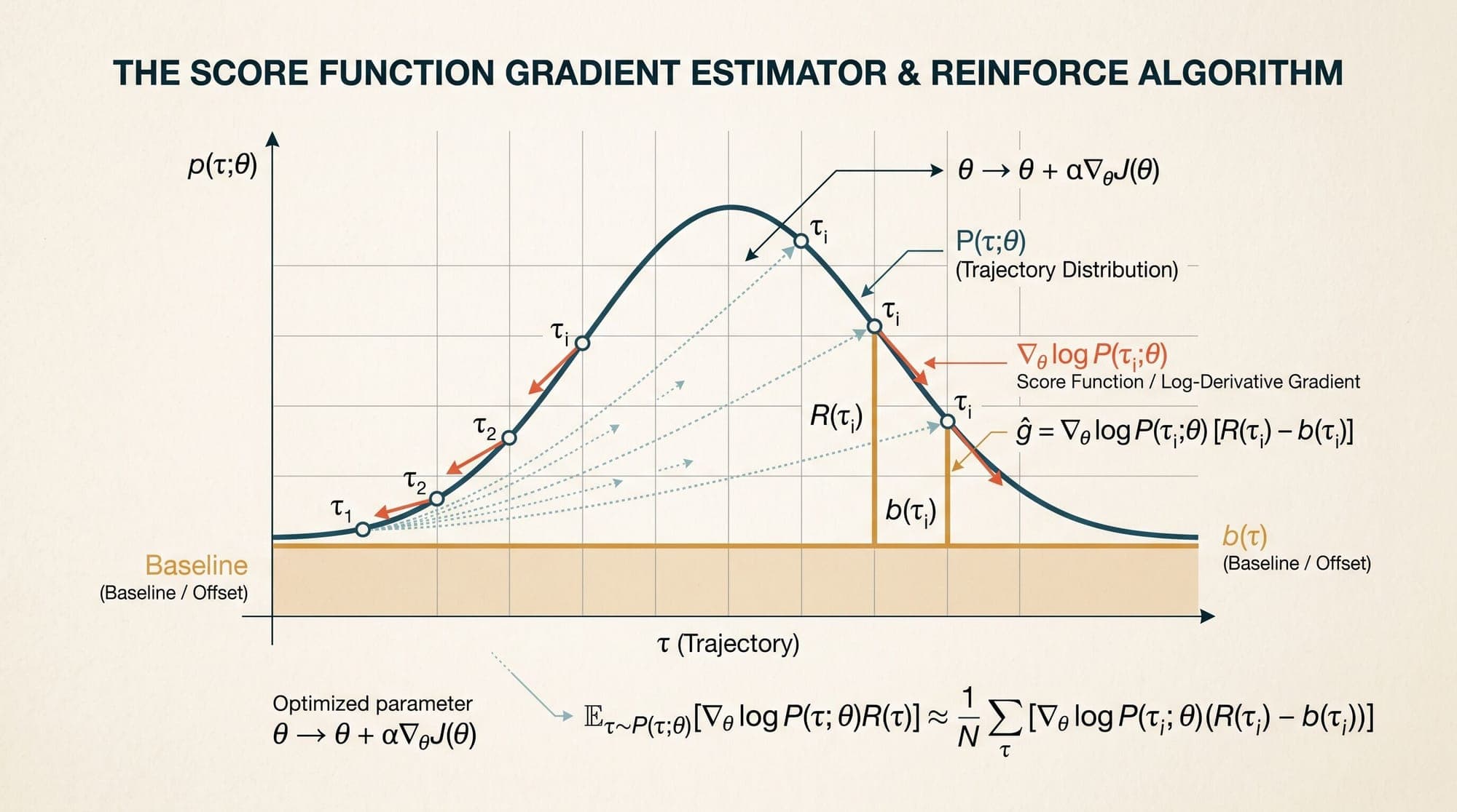
The foundational theoretical engine solving this problem is the score function estimator (historically formalized in reinforcement learning as the REINFORCE algorithm by Ronald J. Williams in 1992). By applying the log-derivative identity (often called the likelihood ratio trick), the score function estimator converts the gradient of an expectation over an intractable or non-differentiable landscape into an expectation of a score-weighted objective.
                    STOCHASTIC GRADIENT ESTIMATION TAXONOMY

                          ∇_θ E_{x ~ p_θ}[f(x)]
                                   │
         ┌─────────────────────────┴─────────────────────────┐
         ▼                                                   ▼
Pathwise Derivative                               Score Function Estimator
(Reparameterization Trick)                        (Likelihood Ratio / REINFORCE)
• x = g(θ, ε), ε ~ p(ε)                           • ∇_θ E[f(x)] = E[f(x) ∇_θ log p_θ(x)]
• Requires differentiable f(x)                     • Operates on arbitrary / black-box f(x)
• Continuous variables only                       • Supports discrete & combinatorial domains
• Low variance Monte Carlo estimates              • High variance; requires baseline reduction
• Used in VAEs, Diffusion Models                  • Used in Policy Gradients, RLHF, GRPO, RLVR
Understanding the exact mathematical derivation of the score function, its connection to the Fisher Information matrix, the necessity of control variates for variance reduction, and its contemporary realization in algorithms like PPO and GRPO is essential for understanding post-training alignment and reasoning systems.
The Mathematical Derivation: The Log-Derivative Identity
Consider an optimization objective defined as the expectation of a scalar performance metric f(x) under a probability density or mass function p_theta(x) parameterized by vector theta in R^d:
J(theta) = E_{x ~ p_theta}[f(x)] = Integral_x p_theta(x) f(x) dx
The goal is to compute the analytical gradient with respect to the distribution parameters, nabla_theta J(theta).
Because the parameter vector theta governs the sampling distribution rather than the function f(x) directly, the gradient operator nabla_theta cannot simply differentiate f(x). Assuming standard regularity conditions (specifically, that p_theta(x) is continuously differentiable with respect to theta and the integral satisfies the Leibniz integral rule under dominated convergence), the gradient passes inside the integral:
nabla_theta J(theta) = nabla_theta Integral_x p_theta(x) f(x) dx = Integral_x nabla_theta p_theta(x) f(x) dx
The integral Integral_x nabla_theta p_theta(x) f(x) dx cannot be directly approximated via standard Monte Carlo sampling because nabla_theta p_theta(x) is generally not a valid probability density function (it integrates to zero rather than one).
To restore an expectation form, multiply and divide the integrand by p_theta(x) wherever p_theta(x) > 0:
nabla_theta J(theta) = Integral_x p_theta(x) [ (nabla_theta p_theta(x)) / p_theta(x) ] f(x) dx
From basic calculus, the derivative of the natural logarithm of a positive function u(theta) is nabla_theta log u(theta) = (nabla_theta u(theta)) / u(theta). Applying this log-derivative identity yields:
(nabla_theta p_theta(x)) / p_theta(x) = nabla_theta log p_theta(x)
Substituting this identity back into the integral produces the fundamental score function gradient equation:
nabla_theta J(theta) = Integral_x p_theta(x) [ f(x) nabla_theta log p_theta(x) ] dx = E_{x ~ p_theta} [ f(x) nabla_theta log p_theta(x) ]
The quantity nabla_theta log p_theta(x) is known in classical statistics as the score function S(theta; x).
nabla_theta J(theta) = E_{x ~ p_theta} [ f(x) S(theta; x) ]
This formulation guarantees that an empirical Monte Carlo estimator computed over N discrete samples x_i ~ p_theta(x):
grad_est = (1 / N) sum_{i=1}^N f(x_i) nabla_theta log p_theta(x_i)
is a strictly unbiased estimator of the true gradient nabla_theta J(theta), regardless of whether f(x) is discontinuous, non-smooth, discrete, or computed by an external physical environment.
Core Statistical Properties of the Score Function
The score function S(theta; x) = nabla_theta log p_theta(x) exhibits mathematical properties that govern both its optimization behavior and variance characteristics.
1. Zero Expected Score
The expectation of the score function under its own parameterized distribution is identically zero:
E_{x ~ p_theta}[nabla_theta log p_theta(x)] = Integral p_theta(x) [ (nabla_theta p_theta(x)) / p_theta(x) ] dx = Integral nabla_theta p_theta(x) dx = nabla_theta Integral p_theta(x) dx = nabla_theta (1) = 0
This zero-mean property is the algebraic foundation that enables unbiased baseline variance reduction.
2. The Fisher Information Matrix
The covariance matrix of the score function defines the Fisher Information Matrix:
I(theta) = Cov[S(theta; x)] = E_{x ~ p_theta} [ (nabla_theta log p_theta(x)) (nabla_theta log p_theta(x))^T ] = -E_{x ~ p_theta} [ nabla_theta^2 log p_theta(x) ]
The Fisher Information matrix characterizes the local curvature of the distribution manifold in parameter space and forms the theoretical basis for natural policy gradients and trust region optimization methods (TRPO and PPO).

Comparing Score Function vs. Pathwise Derivatives
In stochastic computation graphs, two primary paradigms exist for estimating gradients through random variables: the Score Function Estimator (likelihood ratio / REINFORCE) and the Pathwise Derivative (the reparameterization trick introduced by Kingma & Welling in 2013):
- Transformation Formulation: The score function estimator samples directly from x ~ p_theta(x). In contrast, the pathwise derivative reparameterizes x = g(theta, epsilon), where epsilon ~ p(epsilon) is an parameter-free noise source.
- Gradient Expression: Score function computes E[f(x) nabla_theta log p_theta(x)]. Pathwise derivative computes E[nabla_x f(x) nabla_theta g(theta, epsilon)].
- Requirements on f(x): Score function treats f(x) as a black box (supporting discrete, discontinuous, or non-differentiable objectives). Pathwise derivative strictly requires a continuously differentiable objective nabla_x f(x).
- Requirements on Sample Space: Score function supports discrete, combinatorial, and continuous distributions. Pathwise derivative requires continuous and invertible coordinate transforms.
- Estimator Variance: Score function estimates typically suffer from high to extreme variance. Pathwise derivative estimates exhibit low variance because they directly propagate the analytical gradient of f(x).
- Primary Applications: Score function estimators power policy gradients, RLHF, GRPO, and discrete tool use. Pathwise derivatives power Variational Autoencoders (VAEs), continuous diffusion models, and normalizing flows.
When f(x) is smooth and continuous, the pathwise derivative provides superior sample efficiency. However, when x represents discrete categorical decisions (such as token indices in language generation), coordinate transformations are discontinuous, making the score function estimator strictly necessary.
Trajectory-Level Policy Gradients and REINFORCE
In sequential decision-making environments and autoregressive language modeling, actions are not isolated events; they form multi-step trajectories tau = (s_0, a_0, s_1, a_1, ..., s_T, a_T).
Let a policy pi_theta(a_t | s_t) govern action selection, while environment dynamics P(s_{t+1} | s_t, a_t) govern state transitions. The probability distribution over a full trajectory tau is:
P(tau; theta) = mu(s_0) * product_{t=0}^T [ pi_theta(a_t | s_t) P(s_{t+1} | s_t, a_t) ]
The expected cumulative return is J(theta) = E_{tau ~ P(.; theta)} [R(tau)], where R(tau) = sum_{t=0}^T gamma^t r(s_t, a_t).
Applying the score function estimator directly to the trajectory distribution:
nabla_theta J(theta) = E_{tau ~ P(.; theta)} [ R(tau) nabla_theta log P(tau; theta) ]
Expanding the log-probability of the trajectory:
log P(tau; theta) = log mu(s_0) + sum_{t=0}^T log pi_theta(a_t | s_t) + sum_{t=0}^T log P(s_{t+1} | s_t, a_t)
Differentiating with respect to the policy parameters theta:
nabla_theta log P(tau; theta) = sum_{t=0}^T nabla_theta log pi_theta(a_t | s_t)
Notice that the initial state distribution mu(s_0) and the transition dynamics P(s_{t+1} | s_t, a_t) contain no dependence on theta, so their gradients evaluate to zero. This is the central breakthrough of the Policy Gradient Theorem (Sutton et al., 1999): the gradient of expected trajectory reward requires no knowledge of environment transition dynamics.
nabla_theta J(theta) = E_{tau} [ ( sum_{t=0}^T nabla_theta log pi_theta(a_t | s_t) ) R(tau) ]
Enforcing Temporal Causality (Rewards-to-Go)
In the raw trajectory formulation, actions at time step t are multiplied by rewards obtained prior to time t. Because future actions cannot causally affect past rewards, the expectation E[nabla_theta log pi_theta(a_t|s_t) r(s_{t'}, a_{t'})] = 0 for all t' < t. Removing non-causal past terms yields the standard rewards-to-go formulation:
nabla_theta J(theta) = E_{tau} [ sum_{t=0}^T nabla_theta log pi_theta(a_t | s_t) G_t ], where G_t = sum_{t'=t}^T gamma^{t'-t} r(s_{t'}, a_{t'})
This causal truncation reduces estimator variance substantially without introducing any bias.
The Variance Crisis and Control Variates
The primary failure mode of the raw score function estimator is extreme variance. Because the scalar return G_t multiplies the sum of gradient vectors, stochastic variations in trajectory returns introduce noise that scales exponentially with horizon length T. In high-dimensional neural networks, high gradient variance causes destructive parameter updates, erratic learning trajectories, and severe sample inefficiency.
Baseline Subtraction as an Unbiased Control Variate
To mitigate variance, practitioners introduce a baseline function b(s_t) that depends on the state s_t but is strictly independent of the action a_t. The modified gradient estimator is:
nabla_theta J(theta) = E_{tau} [ sum_{t=0}^T nabla_theta log pi_theta(a_t | s_t) (G_t - b(s_t)) ]
Proof of Unbiasedness: We prove that subtracting b(s_t) introduces zero expectation bias by applying the law of iterated expectations:
E_{s_t, a_t} [ nabla_theta log pi_theta(a_t | s_t) b(s_t) ] = E_{s_t} [ b(s_t) E_{a_t ~ pi_theta(.|s_t)} [nabla_theta log pi_theta(a_t | s_t)] ]
From the zero expected score property proven earlier:
E_{a_t ~ pi_theta(.|s_t)} [nabla_theta log pi_theta(a_t | s_t)] = sum_{a_t} pi_theta(a_t|s_t) [ (nabla_theta pi_theta(a_t|s_t)) / pi_theta(a_t|s_t) ] = nabla_theta sum_{a_t} pi_theta(a_t|s_t) = nabla_theta (1) = 0
Therefore:
E_{s_t} [ b(s_t) * 0 ] = 0
Subtracting any state-dependent baseline preserves exact gradient expectation while dramatically reducing the magnitude of the scalar multiplying the score vectors.
                  VARIANCE REDUCTION VIA BASELINE CONTROL VARIATE

   Raw Return Vector:
   G_t = +102.4 ─────────────────────────────────────────► |Large Gradient Step|

   Baseline Offset:
   b(s_t) = +100.0 (Expected state value)

   Advantage Offset:
   A_t = (G_t - b(s_t)) = +2.4 ──► |Tight, Low-Variance Gradient Step|
Derivation of the Optimal Baseline
As analyzed by Greensmith, Bartlett, & Baxter (2004), the variance of the gradient estimator along coordinate k is minimized when the baseline equals:
b_k^*(s) = ( E_{a ~ pi_theta} [ Q(s, a) ( nabla_{theta_k} log pi_theta(a|s) )^2 ] ) / ( E_{a ~ pi_theta} [ ( nabla_{theta_k} log pi_theta(a|s) )^2 ] )
In deep reinforcement learning, computing coordinate-wise optimal baselines is computationally impractical. Instead, setting b(s_t) = V^pi(s_t) = E_{a ~ pi}[Q(s_t, a)] provides near-optimal variance reduction. The resulting centered scalar:
A(s_t, a_t) = Q(s_t, a_t) - V(s_t)
is the Advantage function, measuring how much better a specific action a_t is compared to the expected outcome from state s_t.
The Evolution of Score Function Estimators in Modern LLMs
The mathematical framework of the score function estimator underpins nearly all modern post-training reinforcement learning in frontier language models.
                   EVOLUTION OF SCORE FUNCTION ALGORITHMS

 1992: REINFORCE (Williams)
 │     • Raw score function: ∇_θ E[R] = E[R ∇_θ log π_θ(a|s)]
 │     • High variance; no value network
 ▼
 2017: PPO with Generalized Advantage Estimation (Schulman et al.)
 │     • Clipped surrogate objective prevents destructive policy steps
 │     • Dual network: Actor π_θ and learned Critic V_ϕ(s)
 ▼
 2024: GRPO: Group Relative Policy Optimization (DeepSeekMath)
 │     • Critic-free architecture (saves ~50% GPU memory during training)
 │     • Samples G outputs per prompt: {o_1, o_2, ..., o_G}
 │     • Computes empirical group baseline: b = mean(r_1, ..., r_G)
 │     • Advantage: A_i = (r_i - mean(r)) / std(r)
 ▼
 2025-2026: RLVR: Reinforcement Learning with Verifiable Rewards
       • Pure deterministic execution oracles (compilers, formal math verifiers)
       • Binary reward signals r in {0, 1} scaled via group score estimators
1. Proximal Policy Optimization (PPO)
Standard LLM RLHF frameworks implement PPO (Schulman et al., 2017), maintaining a parameterized policy pi_theta (the generative language model) and a separate value network V_phi (the critic). The score function gradient is modified using an importance-sampling ratio r_t(theta) = (pi_theta(a_t|s_t)) / (pi_{theta_old}(a_t|s_t)) and a pessimistic clipping operator:
L^{CLIP}(theta) = E_t [ min( r_t(theta) hat{A}_t, clip(r_t(theta), 1-epsilon, 1+epsilon) hat{A}_t ) ]
where hat{A}_t is estimated using Generalized Advantage Estimation (GAE).
2. Group Relative Policy Optimization (GRPO)
While PPO effectively suppresses variance, maintaining a separate value network V_phi with equal parameter scale to the policy doubles memory consumption and communication overhead during distributed training.
To solve this, DeepSeek introduced Group Relative Policy Optimization (GRPO) for mathematical and reasoning post-training. GRPO eliminates the critic network entirely by sampling a group of G responses {o_1, o_2, ..., o_G} for each query prompt q.
The baseline is computed directly from the group reward distribution:
r_mean = (1 / G) sum_{i=1}^G r_i, sigma_r = sqrt( (1 / G) sum_{i=1}^G (r_i - r_mean)^2 + epsilon )
The advantage for each response is standardized:
hat{A}_i = (r_i - r_mean) / sigma_r
GRPO uses the group mean as a sample-based control variate baseline. Because the group mean is computed across outputs generated by the same policy under the same prompt condition, it provides unbiased variance reduction without allocating GPU memory for a value network.
3. Reinforcement Learning with Verifiable Rewards (RLVR)
In complex reasoning tasks (coding, mathematics, and logic proofs), human preference reward models suffer from reward hacking and calibration drift. Frontier architectures increasingly use Reinforcement Learning with Verifiable Rewards (RLVR).
Under RLVR:
- f(x) is a deterministic verification oracle (such as passing a pytest suite, executing Python code in a sandbox, or checking a Lean 4 formal proof).
- The reward is strictly binary: r(x) in {0, 1}.
- The score function estimator adjusts token logits along trajectories that successfully compile and solve the verification test case, while penalizing failed branches relative to the group baseline.
Summary and Architectural Takeaways
The score function gradient estimator bridges continuous optimization and discrete probabilistic execution:
- Analytical Mechanics: By rewriting nabla_theta p_theta(x) as p_theta(x) nabla_theta log p_theta(x), the log-derivative trick enables gradient estimation over arbitrary non-differentiable or black-box reward functions without requiring backpropagation through environment dynamics.
- Variance Scaling: Raw score function estimates suffer from variance that compounds with trajectory length. Variance reduction is mathematically essential and achieved by subtracting action-independent baselines b(s), which contribute zero expected bias due to the zero-mean property of the score function.
- From Dual Networks to Group Baselines: While actor-critic architectures (PPO) historically relied on auxiliary value models to estimate state baselines, modern frontier reasoning pipelines (GRPO and RLVR) achieve comparable variance reduction by utilizing multi-sample group baselines, slashing memory requirements while scaling discrete reasoning performance.
Sources
- Williams, R. J. (1992). Simple statistical gradient-following algorithms for connectionist reinforcement learning. Machine Learning, 8(3-4), 229-256. DOI: 10.1007/BF00992696
- Sutton, R. S., McAllester, D., Singh, S., & Mansour, Y. (1999). Policy Gradient Methods for Reinforcement Learning with Function Approximation. Advances in Neural Information Processing Systems (NeurIPS 1999). NeurIPS Proceedings
- Greensmith, E., Bartlett, P. L., & Baxter, J. (2004). Variance Reduction Techniques for Gradient Estimates in Reinforcement Learning. Journal of Machine Learning Research (JMLR), 5, 1471-1530. JMLR Paper
- Kingma, D. P., & Welling, M. (2013). Auto-Encoding Variational Bayes. arXiv:1312.6114. arXiv:1312.6114
- Schulman, J., Wolski, F., Dhariwal, P., Radford, A., & Klimov, O. (2017). Proximal Policy Optimization Algorithms. arXiv:1707.06347. arXiv:1707.06347
- Shao, Z., et al. (2024). DeepSeekMath: Pushing the Limits of Mathematical Reasoning in Open Language Models. arXiv:2402.03300. arXiv:2402.03300
- DeepSeek-AI. (2025). DeepSeek-R1: Incentivizing Reasoning Capability in LLMs via Reinforcement Learning. arXiv:2501.12948. arXiv:2501.12948



