Pipeline Parallelism in Large Language Models: How GPipe, 1F1B Scheduling, and Interleaving Tame Memory and Bubbles

Training frontier large language models with tens or hundreds of billions of parameters exceeds the physical memory capacity of any individual GPU. While intra-node sharding strategies such as Tensor Parallelism partition individual matrix multiplications across accelerators over high-speed NVLink interconnects, scaling across multi-node clusters encounters strict hardware boundaries.

Tensor Parallelism requires multiple collective All-Reduce communications per transformer layer. Across standard cluster networking fabrics, such as InfiniBand or RoCE, the latency and bandwidth penalty of cross-node All-Reduce operations collapses training throughput. Meanwhile, standard Data Parallelism and Fully Sharded Data Parallelism (FSDP) incur recurring All-Gather and Reduce-Scatter collective overheads across all ranks.

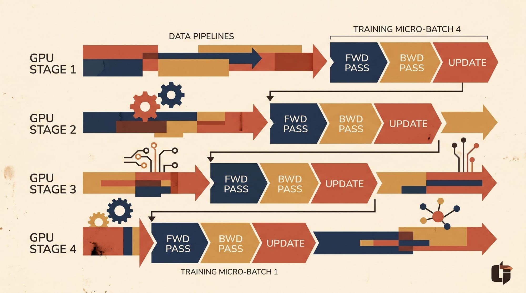
Pipeline Parallelism (PP) resolves this multi-node scaling constraint by partitioning neural networks along their depth. Rather than splitting individual weight matrices within a layer, Pipeline Parallelism places consecutive sequences of transformer layers onto distinct accelerator stages. Communication between stages is strictly point-to-point, transferring only the boundary activations during the forward pass and activation gradients during the backward pass.

The Pipeline Bubble and GPipe Scheduling

The fundamental challenge in pipeline parallelism is device idle time, known as the pipeline bubble. In a naive execution where a single batch is processed sequentially through $P$ pipeline stages, only one stage is active at any given moment. The remaining $P - 1$ stages sit completely idle while waiting for inputs from upstream stages during the forward pass or gradients from downstream stages during backpropagation.

To overcome this latency stall, Google Brain introduced GPipe (Huang et al., 2019). GPipe subdivides a global training batch into $M$ smaller, independent micro-batches ($M \gg P$). The first stage computes the forward pass on micro-batch 0 and immediately transmits the resulting activations to stage 1. While stage 1 executes micro-batch 0, stage 0 begins computing micro-batch 1.

Under the standard GPipe schedule (often called the Flush or Forward-then-Backward schedule):

• Forward Phase: Each stage processes all $M$ forward micro-batches sequentially, forwarding activation tensors downstream.
• Backward Phase: Once the final stage computes the loss for all micro-batches, backpropagation begins in reverse order, passing activation gradients back upstream.

While micro-batching dramatically improves hardware concurrency compared to naive sequential execution, GPipe suffers from two major structural constraints:

1. Bubble Overhead: During the start of the forward pass (pipeline fill) and the end of the backward pass (pipeline drain), stages experience compulsory idle time. For $P$ pipeline stages and $M$ micro-batches, the total bubble time across all stages is $(P - 1) \cdot (t_F + t_B)$, where $t_F$ is forward execution time per micro-batch and $t_B$ is backward execution time. Assuming $t_B \approx 2 t_F$, the theoretical pipeline bubble fraction $F_{\text{bubble}}$ is:

$$F_{\text{bubble}} = \frac{P - 1}{M + P - 1}$$

To reduce the bubble fraction to an acceptable level (such as under 10%), distributed training systems must set $M \ge 8P$ or $M \ge 16P$.

1. Activation Memory Explosion: Because GPipe executes all $M$ forward passes before executing any backward passes, each stage must preserve the intermediate activation tensors for all $M$ micro-batches in GPU VRAM. As operators increase $M$ to suppress the pipeline bubble, peak activation memory scales linearly with $M$. For large models, this memory footprint triggers out-of-memory errors, restricting the maximum number of micro-batches that can be evaluated.

The 1F1B Schedule: Decoupling Memory from Micro-Batch Count

To break the linear coupling between micro-batch count and activation memory, the One-Forward-One-Backward (1F1B) schedule was proposed in PipeDream (Narayanan et al., 2019) and adapted for synchronous distributed LLM training in Megatron-LM (Narayanan et al., 2021).

Rather than accumulating all forward passes before beginning backpropagation, the 1F1B schedule transitions stages into an alternating steady state:

• Warmup Phase: Stage $i$ executes $P - i - 1$ forward micro-batches. This primes downstream stages with initial activations.
• Steady-State Phase: Each stage executes exactly one backward micro-batch (which computes gradients and frees that micro-batch's cached activation memory) for every one forward micro-batch it accepts.
• Cooldown Phase: Once all $M$ forward micro-batches have completed, each stage drains its remaining outstanding backward micro-batches.

The mathematical advantage of 1F1B lies in its peak memory bound. In 1F1B, the maximum number of in-flight forward activations stored in memory on any stage is strictly capped at the pipeline depth $P$, completely independent of the total micro-batch count $M$.

This bounded memory property allows engineering teams to scale $M$ to large values (such as $M = 32$ or $M = 64$) to dilute the pipeline bubble without increasing the per-GPU activation memory footprint.

Interleaved 1F1B: Virtual Stages for Tighter Schedules

While standard 1F1B bounds peak activation memory, the bubble fraction remains $(P - 1) / (M + P - 1)$. In large clusters requiring deep pipelines ($P = 16$ or $P = 32$), achieving a small bubble fraction demands very large values of $M$. However, total batch size equals $M \times \text{micro-batch size} \times \text{Data Parallel size}$. If $M$ is forced to be large, the global batch size can exceed the optimal statistical convergence threshold for LLM pretraining.

To address this limitation, the Megatron-LM team introduced the Interleaved 1F1B schedule (Narayanan et al., 2021). In this paradigm, each physical GPU hosts $v$ virtual stages (chunks) distributed across the model depth rather than a single contiguous block of layers.

For instance, with $P = 4$ physical devices and a virtual chunk factor of $v = 2$:

• Device 0 holds Chunk 0 (Layers 1-4) and Chunk 4 (Layers 17-20).
• Device 1 holds Chunk 1 (Layers 5-8) and Chunk 5 (Layers 21-24).
• Device 2 holds Chunk 2 (Layers 9-12) and Chunk 6 (Layers 25-28).
• Device 3 holds Chunk 3 (Layers 13-16) and Chunk 7 (Layers 29-32).

Because each virtual stage processes fewer layers, activations circulate through physical devices in shorter cycles. The resulting pipeline bubble fraction is reduced by a factor of $v$:

$$F_{\text{bubble, interleaved}} \approx \frac{1}{v} \cdot \frac{P - 1}{M}$$

For example, using $v = 2$ cuts the pipeline bubble duration approximately in half for a given micro-batch count $M$. The trade-off is communication frequency: interleaving increases point-to-point peer network transfers by a factor of $v$, requiring sufficient network bandwidth between adjacent pipeline stages.

Zero-Bubble Pipeline Parallelism: Decoupling Weight and Activation Gradients

Even with interleaving, synchronous pipeline schedules historically faced a theoretical bubble lower bound determined by dependency graphs. In 2024, researchers from Sea AI Lab introduced Zero Bubble Pipeline Parallelism (Qi et al., 2024), demonstrating that pipeline bubbles can be reduced to near-zero while preserving exact synchronous training semantics.

Zero-Bubble scheduling exploits a fundamental mathematical property of backpropagation in neural network layers. The backward pass consists of two independent tensor computations:

1. Activation Gradient ($B$ or $\nabla_x$): Computes the gradient of the loss with respect to the input activations. This tensor is on the critical execution path because it must be transmitted immediately to the upstream pipeline stage so that earlier layers can continue backpropagation.
2. Parameter Gradient ($W$ or $\nabla_w$): Computes the gradient of the loss with respect to layer weights. This tensor is not required by any other pipeline stage; it only needs to be accumulated locally prior to the final optimizer step.

In standard 1F1B, $B$ and $W$ are computed together in an atomic backward operation. Zero-Bubble algorithms (such as ZB1P, ZB2P, and ZBV) split backward execution into separate $B$ and $W$ tasks.

By executing $B$ passes with high priority to unblock upstream stages and deferring $W$ passes into the idle time slots of the warmup and cooldown phases, the scheduler fills the pipeline bubbles with useful parameter gradient computation. In empirical benchmarks on Megatron-LM, Zero-Bubble schedules deliver up to 20% to 30% higher training throughput compared to standard 1F1B under equivalent memory budgets.

3D Parallelism Topology and Production Deployment

In production distributed training clusters (such as Megatron-DeepSpeed and PyTorch FSDP setups), Pipeline Parallelism is rarely deployed in isolation. Instead, it forms the third dimension of 3D parallelism:

• Tensor Parallelism (TP, intra-node): Applied within single 8-GPU servers over high-bandwidth NVLink (900 GB/s to 1.8 TB/s). TP splits attention heads and MLP hidden dimensions where low-latency communication is mandatory.
• Pipeline Parallelism (PP, inter-node): Applied across multi-node boundaries over standard InfiniBand/RoCE fabrics. Because PP only transmits boundary activations and activation gradients ($O(B \cdot s \cdot h)$ per micro-batch), it operates efficiently across lower-bandwidth cross-node networks.
• Data Parallelism / FSDP (DP, cluster-wide): Replicates the TP+PP model pipeline across orthogonal GPU groups, performing asynchronous gradient reductions across pipeline replicas.

By combining intra-node Tensor Parallelism with bounded 1F1B or Zero-Bubble Pipeline Parallelism across nodes, distributed training clusters can scale foundation models to trillions of parameters while maintaining high Model Flops Utilization (MFU).

Sources

• GPipe: Efficient Training of Giant Neural Networks using Pipeline Parallelism (Huang et al., 2019)
• PipeDream: Generalized Pipeline Parallelism for DNN Training (Narayanan et al., 2019)
• Efficient Large-Scale Language Model Training on GPU Clusters Using Megatron-LM (Narayanan et al., 2021)
• Zero Bubble Pipeline Parallelism (Qi et al., 2024)
• PyTorch FSDP: Experiences on Scaling Fully Sharded Data Parallel (Zhao et al., 2023)