Performers and FAVOR+: How Positive Orthogonal Random Features Linearize Transformer Attention

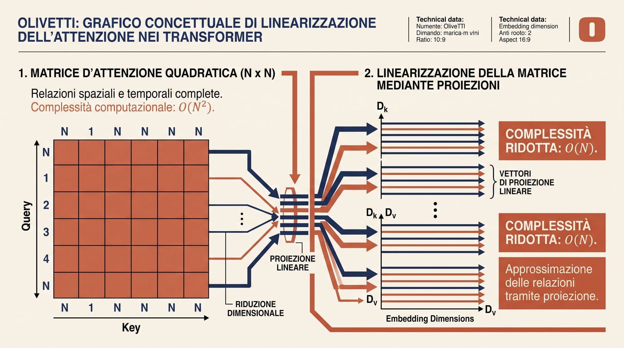
The quadratic complexity of standard self-attention has remained a central computational ceiling in Transformer architectures. Because standard attention computes pairwise similarity across all token pairs in a sequence of length $L$, memory consumption and compute scale as $O(L^2)$. For long contexts, high-resolution visual tokens, and biological sequence modeling, this quadratic bottleneck forces strict sequence truncation or aggressive hardware partitioning.

In Rethinking Attention with Performers, Choromanski et al. (2020) introduced the Performer architecture powered by FAVOR+ (Fast Attention Via Positive Orthogonal Random Features). Unlike low-rank approximations or sparse attention patterns that alter the model's receptive field, FAVOR+ establishes an unbiased, low-variance mathematical estimator of the full-rank softmax attention matrix that operates in $O(L)$ linear time and space.

1. The Quadratic Bottleneck in Scaled Dot-Product Attention

Standard scaled dot-product attention, formalized by Vaswani et al. (2017), maps queries $Q \in \mathbb{R}^{L \times d}$, keys $K \in \mathbb{R}^{L \times d}$, and values $V \in \mathbb{R}^{L \times d_{\text{val}}}$ through an explicit attention matrix $A$:

$$\text{Attn}(Q, K, V) = D^{-1} A V$$

where the raw affinity matrix $A \in \mathbb{R}^{L \times L}$ and the normalizer diagonal matrix $D \in \mathbb{R}^{L \times L}$ are defined as:

$$A = \exp\left(\frac{Q K^T}{\sqrt{d}}\right), \quad D = \text{diag}(A \mathbf{1}_L)$$

Here, $\exp(\cdot)$ denotes element-wise exponentiation and $\mathbf{1}_L$ is an all-ones column vector of length $L$.

The quadratic cost stems directly from the matrix product $Q K^T$. Constructing $A$ requires calculating $L^2$ pairwise inner products and storing an $L \times L$ activation map in GPU memory for the backward pass. Because softmax normalizes rows after exponentiation, the operations cannot be rearranged using standard matrix associativity:

$$(Q K^T) V \neq Q (K^T V)$$

If $A$ could be factored into the product of two low-dimensional feature representations, $A \approx Q' (K')^T$ where $Q', K' \in \mathbb{R}^{L \times M}$ with $M \ll L$, matrix associativity would allow computing $(K')^T V \in \mathbb{R}^{M \times d_{\text{val}}}$ first in $O(L M d_{\text{val}})$ time, followed by left-multiplication by $Q'$ in $O(L M d_{\text{val}})$ time.

2. Attention as a Continuous Kernel Evaluation

To linearize the attention mechanism without restricting the attention matrix rank, Choromanski et al. (2020) reframed attention elements as continuous kernel evaluations. For a query vector $q_i \in \mathbb{R}^d$ and a key vector $k_j \in \mathbb{R}^d$, the unnormalized attention affinity is:

$$\text{Ker}(q_i, k_j) = \exp\left(\frac{q_i^T k_j}{\sqrt{d}}\right)$$

By defining scaled vectors $x = q_i / d^{1/4}$ and $y = k_j / d^{1/4}$, the kernel simplifies to the generalized exponential kernel:

$$K_{\text{exp}}(x, y) = \exp(x^T y)$$

Under classic kernel theory, any positive definite kernel $K(x, y)$ can be decomposed as an inner product in a high-dimensional feature space $\mathcal{H}$:

$$K(x, y) = \langle \Phi(x), \Phi(y) \rangle_{\mathcal{H}} = \mathbb{E}_{\omega}\left[ \phi(x; \omega)^T \phi(y; \omega) \right]$$

where $\phi(\cdot; \omega): \mathbb{R}^d \to \mathbb{R}^M$ represents a randomized feature mapping parameterized by random vector $\omega$. If an empirical estimator $\hat{K}(x, y) = \phi(x)^T \phi(y)$ provides an unbiased approximation of $\exp(x^T y)$, the full attention computation becomes:

$$\text{Attn}(Q, K, V)_i = \frac{\sum_{j=1}^L \phi(q_i)^T \phi(k_j) v_j}{\sum_{j=1}^L \phi(q_i)^T \phi(k_j)} = \frac{\phi(q_i)^T \sum_{j=1}^L \phi(k_j) v_j^T}{\phi(q_i)^T \sum_{j=1}^L \phi(k_j)}$$

By pulling the query feature $\phi(q_i)^T$ outside the summation over sequence index $j$, the key and value interactions can be pre-aggregated across the entire sequence into a global context tensor $S = \sum_{j=1}^L \phi(k_j) v_j^T \in \mathbb{R}^{M \times d_{\text{val}}}$ and a normalizer vector $z = \sum_{j=1}^L \phi(k_j) \in \mathbb{R}^M$.

3. Why Random Fourier Features Fail for Softmax Attention

Approximating shift-invariant kernels via randomized features was pioneered by Rahimi and Recht (2007) using Random Fourier Features (RFF). For a standard Gaussian radial basis function (RBF) kernel $K_{\text{gauss}}(x, y) = \exp(-\|x - y\|^2 / 2)$, Bochner's Theorem guarantees that the Fourier transform of the kernel is a valid probability distribution $\mathcal{N}(0, I_d)$.

The exponential kernel can be rewritten in terms of the Gaussian kernel:

$$\exp(x^T y) = \exp\left(-\frac{\|x - y\|^2}{2}\right) \exp\left(\frac{\|x\|^2 + \|y\|^2}{2}\right) = K_{\text{gauss}}(x, y) \exp\left(\frac{\|x\|^2}{2}\right) \exp\left(\frac{\|y\|^2}{2}\right)$$

Applying trigonometric Random Fourier Features to approximate $K_{\text{gauss}}(x, y)$ yields the trigonometric mapping:

$$\phi_{\text{trig}}(x) = \frac{\exp(\|x\|^2 / 2)}{\sqrt{M}} \left[ \cos(\omega_1^T x), \sin(\omega_1^T x), \dots, \cos(\omega_M^T x), \sin(\omega_M^T x) \right]^T$$

where $\omega_m \sim \mathcal{N}(0, I_d)$.

While $\mathbb{E}[\phi_{\text{trig}}(x)^T \phi_{\text{trig}}(y)] = \exp(x^T y)$ is mathematically unbiased, trigonometric features exhibit severe failure modes when applied to self-attention:

1. Negative Affinity Estimates: Because cosine and sine fluctuate across $[-1, 1]$, the inner product $\phi_{\text{trig}}(x)^T \phi_{\text{trig}}(y)$ can evaluate to negative values. The true softmax kernel is strictly positive ($\exp(x^T y) > 0$).
2. Normalizer Collapse and Division by Zero: When summing over sequence length $L$, the denominator $\sum_{j=1}^L \phi_{\text{trig}}(q_i)^T \phi_{\text{trig}}(k_j)$ can approach zero or turn negative, causing numerical singularity, gradient explosions, and training divergence.
3. High Variance in Tails: For large queries and keys where $x^T y$ is large, the variance of $\phi_{\text{trig}}$ scales exponentially with $\|x\|^2 + \|y\|^2$, requiring an impractical number of random features ($M \gg 10^3$) to stabilize training.

4. Positive Random Features (PRF)

To overcome the catastrophic instability of trigonometric projections, Choromanski et al. (2020) constructed Positive Random Features (PRF).

Consider the moment-generating function of a standard multivariate Gaussian variable $\omega \sim \mathcal{N}(0, I_d)$. For any deterministic vector $u \in \mathbb{R}^d$:

$$\mathbb{E}_{\omega \sim \mathcal{N}(0, I_d)}\left[ \exp(\omega^T u) \right] = \exp\left(\frac{\|u\|^2}{2}\right)$$

Setting $u = x + y$, the expectation expands as:

$$\mathbb{E}_{\omega}\left[ \exp(\omega^T (x + y)) \right] = \exp\left(\frac{\|x + y\|^2}{2}\right) = \exp\left(\frac{\|x\|^2 + \|y\|^2 + 2 x^T y}{2}\right)$$

Rearranging terms to isolate $\exp(x^T y)$ yields the identity:

$$\exp(x^T y) = \exp\left(-\frac{\|x\|^2}{2}\right) \mathbb{E}_{\omega \sim \mathcal{N}(0, I_d)}\left[ \exp(\omega^T x) \exp(\omega^T y) \right] \exp\left(-\frac{\|y\|^2}{2}\right)$$

Because the expectations and scalar exponential factors distribute linearly, the product can be combined under a single expectation:

$$\exp(x^T y) = \mathbb{E}_{\omega \sim \mathcal{N}(0, I_d)}\left[ \exp\left(\omega^T x - \frac{\|x\|^2}{2}\right) \exp\left(\omega^T y - \frac{\|y\|^2}{2}\right) \right]$$

This gives the positive random feature map $\phi_{\text{pos}}(x): \mathbb{R}^d \to \mathbb{R}_{>0}^M$:

$$\phi_{\text{pos}}(x) = \frac{1}{\sqrt{M}} \exp\left(-\frac{\|x\|^2}{2}\right) \begin{bmatrix} \exp(\omega_1^T x) \\ \exp(\omega_2^T x) \\ \vdots \\ \exp(\omega_M^T x) \end{bmatrix}$$

Because the exponential function maps real numbers strictly to positive values ($\exp(z) > 0$ for all $z \in \mathbb{R}$), every entry of $\phi_{\text{pos}}(x)$ is strictly positive. Consequently:

$$\phi_{\text{pos}}(q_i)^T \phi_{\text{pos}}(k_j) > 0 \quad \forall q_i, k_j \in \mathbb{R}^d$$

This guarantees that all estimated attention weights and sequence normalizers remain strictly positive, eliminating division-by-zero singularities without heuristic thresholding or epsilon padding.

Standard Softmax Attention (O(L^2) Complexity):
  Q (L x d) ---> [ Q * K^T ] (L x L) ---> Softmax ---> [ Attn * V ] (L x d_val)
                    |
              Quadratic Memory & Compute Bottleneck

FAVOR+ Linear Attention (O(L * M) Complexity):
  Q (L x d) ---> phi(Q) (L x M) ---\
                                    \---> [ phi(Q) * (phi(K)^T * V) ] (L x d_val)
  K (L x d) ---> phi(K) (L x M) ----/              \
  V (L x d_val) ----------------------------------- Context Tensor S (M x d_val)

5. Orthogonal Random Features (ORF)

While positive random features eliminate negative attention weights, sampling $\omega_1, \dots, \omega_M$ independently from $\mathcal{N}(0, I_d)$ introduces estimation variance. If two sampled vectors $\omega_i$ and $\omega_j$ are nearly collinear, they provide redundant information while failing to cover orthogonal subspaces of $\mathbb{R}^d$.

To minimize estimator variance, FAVOR+ incorporates Orthogonal Random Features (ORF), extending techniques by Yu et al. (2016).

Instead of independent Gaussian sampling, the projection matrix $W \in \mathbb{R}^{M \times d}$ (where $M = b \cdot d$ for integer block count $b$) is constructed in blocks of $d \times d$ orthogonal matrices:

1. Sample a random Gaussian matrix $G \in \mathbb{R}^{d \times d}$ with entries $G_{i,j} \sim \mathcal{N}(0, 1)$.
2. Apply QR decomposition $G = Q_{\text{orth}} R$, where $Q_{\text{orth}} \in \mathbb{R}^{d \times d}$ is an exact orthogonal matrix ($Q_{\text{orth}}^T Q_{\text{orth}} = I_d$).
3. Scale each row of $Q_{\text{orth}}$ by an independent radial sample from the chi-distribution with $d$ degrees of freedom: $S_{\text{diag}} = \text{diag}(\chi_1(d), \dots, \chi_d(d))$.
4. Set the block projection matrix to $W_{\text{block}} = S_{\text{diag}} Q_{\text{orth}}$.

Stacking $b$ such orthogonal blocks yields $W \in \mathbb{R}^{M \times d}$. By enforcing strict orthogonality among rows within each block ($\omega_i^T \omega_j = 0$ for $i \neq j$), ORFs maintain the exact marginal distribution $\mathcal{N}(0, I_d)$ for every individual vector while ensuring that feature dimensions do not duplicate directional coverage.

Choromanski et al. (2020) proved that Orthogonal Positive Random Features strictly reduce the mean squared error (MSE) of the kernel estimator across all sequence lengths compared to standard i.i.d. random features, enabling Performers to achieve high approximation fidelity with relatively small feature counts ($M \in [d, 4d]$).

6. Causal Masking and Recurrent $O(1)$ Inference

In autoregressive language models, tokens must not attend to future positions. The attention output for position $i$ must only incorporate keys and values from indices $j \le i$:

$$\text{Attn}_{\text{causal}}(Q, K, V)_i = \frac{\sum_{j=1}^i \phi(q_i)^T \phi(k_j) v_j}{\sum_{j=1}^i \phi(q_i)^T \phi(k_j)} = \frac{\phi(q_i)^T \left( \sum_{j=1}^i \phi(k_j) v_j^T \right)}{\phi(q_i)^T \left( \sum_{j=1}^i \phi(k_j) \right)}$$

This formulation unlocks two structural computational efficiencies:

Parallel Prefix Sums During Training

The cumulative sum terms:

$$S_i = \sum_{j=1}^i \phi(k_j) v_j^T \in \mathbb{R}^{M \times d_{\text{val}}}, \quad z_i = \sum_{j=1}^i \phi(k_j) \in \mathbb{R}^M$$

can be computed across all $L$ tokens simultaneously using a parallel prefix scan (cumsum) in $O(L M d_{\text{val}})$ time. This maintains parallel training throughput without instantiating lower-triangular $L \times L$ attention masks.

$O(1)$ Memory and Step Latency During Autoregressive Generation

During token-by-token generation, standard Transformers store all past key and value vectors in an expanding KV cache, requiring $O(L)$ memory and $O(L)$ compute per step.

In a Performer, the context state updates recurrently:

$$S_t = S_{t-1} + \phi(k_t) v_t^T$$

$$z_t = z_{t-1} + \phi(k_t)$$

The output for token $t$ is computed in constant time:

$$y_t = \frac{\phi(q_t)^T S_t}{\phi(q_t)^T z_t}$$

The memory footprint during generation is strictly bounded by the fixed state size of $S_t \in \mathbb{R}^{M \times d_{\text{val}}}$ and $z_t \in \mathbb{R}^M$, scaling as $O(M d_{\text{val}})$ regardless of sequence length.

7. Comparison: Standard Attention vs. Linear Attention Variants

| Metric / Property | Standard Softmax Attention | Linear Attention (Katharopoulos et al.) | Performer (FAVOR+) | | :--- | :--- | :--- | :--- | | Kernel Function | $\exp(q^T k / \sqrt{d})$ | $\text{elu}(q) + 1, \text{elu}(k) + 1$ | Unbiased $\exp(q^T k / \sqrt{d})$ Estimator | | Training Time Complexity | $O(L^2 d)$ | $O(L M d)$ | $O(L M d)$ | | Training Space Complexity | $O(L^2 + L d)$ | $O(L M + M d)$ | $O(L M + M d)$ | | Inference Step Complexity | $O(L d)$ | $O(M d)$ | $O(M d)$ | | KV Cache Growth | Linear ($O(L d)$) | Constant ($O(M d)$) | Constant ($O(M d)$) | | Pretrained Softmax Transfer | Native baseline | Requires retraining from scratch | Fine-tunable from pretrained weights |

8. Architectural Trade-Offs and Legacy

While FAVOR+ established the theoretical foundation for provably unbiased linear attention, production deployments navigate specific engineering trade-offs:

1. Random Feature Budget vs. Softmax Fidelity: Approximating sharp softmax distributions with high concentration requires larger feature dimensions $M$. While $M = 256$ is sufficient for many language and biological modeling tasks, highly localized attention patterns can experience minor diffusion compared to exact softmax.
2. Periodic Projection Resampling: In long training runs, drawing static orthogonal random projections $W$ at initialization can cause slight drift. Resampling $W$ periodically during training ensures uniform coverage of activation distributions across training steps.
3. Hardware Alignment: Standard attention implementations benefit from heavily optimized hardware kernels such as FlashAttention that execute fused online softmax directly within GPU SRAM. Because FAVOR+ replaces dense matrix multiplications with multi-step prefix scans, its latency advantage emerges primarily at long sequence lengths ($L \ge 4096$) where memory bandwidth dominates computation.

The mathematical formulation of FAVOR+ provided the bridge between kernel theory, randomized linear algebra, and deep learning. Its principles of associative state accumulation directly influenced subsequent linear attention architectures, state space models (SSMs) like Mamba, and modern recurrent sequence models.

Sources

• Choromanski et al. (2020): Rethinking Attention with Performers
• Google Research: Rethinking Attention with Performers
• Rahimi and Recht (2007): Random Features for Large-Scale Kernel Machines
• Yu et al. (2016): Orthogonal Random Features
• Katharopoulos et al. (2020): Transformers are RNNs: Fast Autoregressive Transformers with Linear Attention
• Vaswani et al. (2017): Attention Is All You Need
• Dao et al. (2022): FlashAttention: Fast and Memory-Efficient Exact Attention with IO-Awareness