Loss Landscapes in Deep Neural Networks: How Filter Normalization, Hessian Curvature, and Basin Flatness Explain Generalization

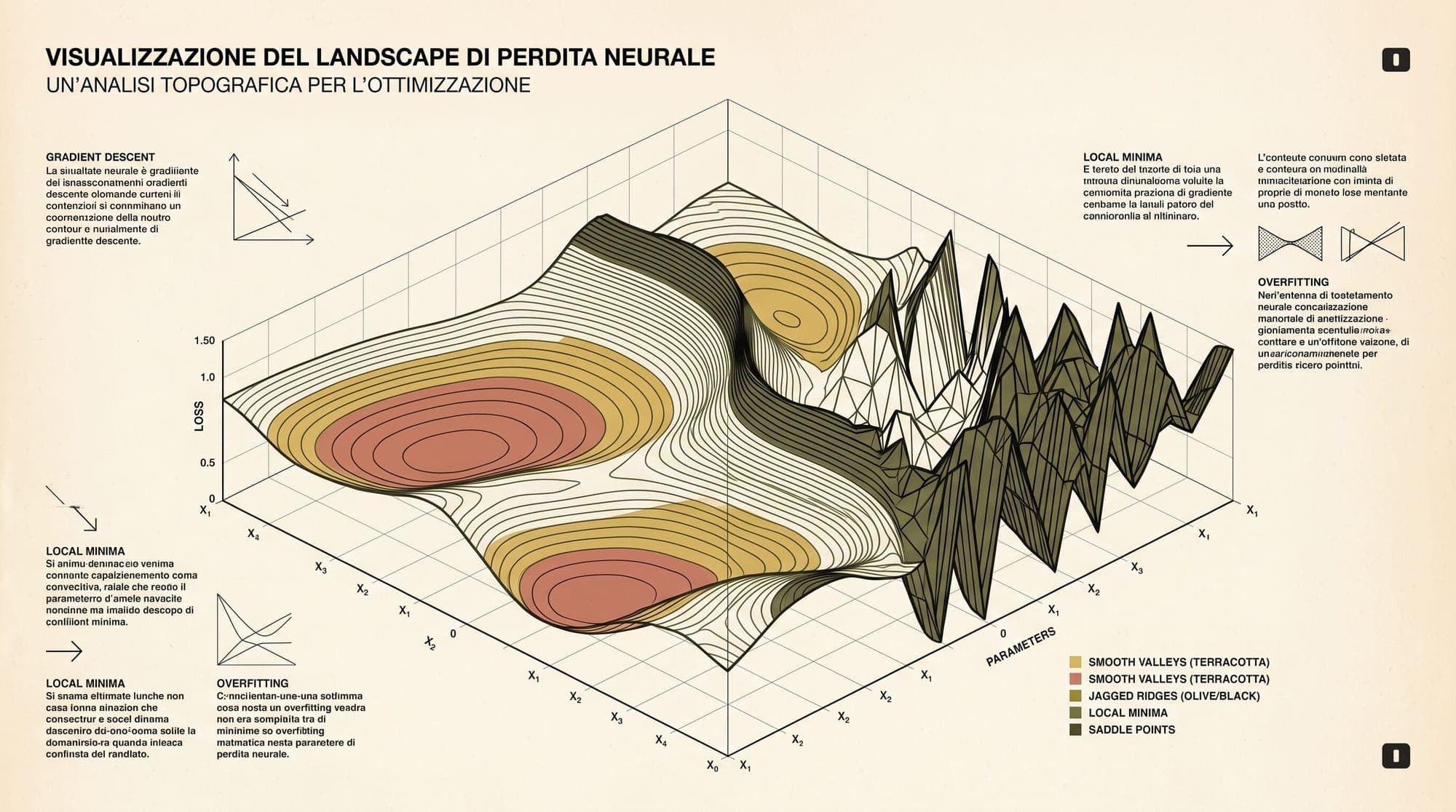
The parameter space of modern deep learning models spans millions to hundreds of billions of dimensions. In this high-dimensional space, the empirical risk objective forms a complex geometric surface known as the loss landscape. Despite the extreme non-convexity of deep neural networks, standard first-order optimization algorithms such as stochastic gradient descent (SGD) and Adam regularly converge to parameter configurations that achieve both low training error and robust test set generalization.

Understanding why neural networks generalize requires analyzing the geometric topography surrounding local minimizers. For decades, visualizing and quantifying these high-dimensional manifolds remained problematic due to scale-invariance artifacts, where arbitrary parameter re-scalings distorted geometric measurements. The development of filter-normalized projection techniques, combined with spectral analysis of the Hessian matrix, has resolved these measurement paradoxes and revealed how network architecture, skip connections, and normalization layers govern the trainability and generalization capacity of deep neural networks.

1. The High-Dimensional Optimization Problem

Given a dataset of input-output pairs and a neural network parameterized by weight vector $\theta \in \mathbb{R}^D$, empirical risk minimization seeks to find:

$$\mathcal{L}(\theta) = \frac{1}{N} \sum_{i=1}^N \ell(f(x_i; \theta), y_i)$$

where $\ell(\cdot, \cdot)$ is a task-specific loss function, such as cross-entropy loss or mean squared error.

In classical non-convex optimization, high-dimensional objective functions are prone to pathological local minima, poor conditioning, and exponential numbers of saddle points. However, deep neural networks exhibit unique geometric characteristics:

• Saddle point abundance over bad local minima: In high dimensions, local minima where all eigenvalues of the Hessian are strictly positive almost exclusively reside near the global minimum risk level, while higher-energy critical points are overwhelmingly saddle points with negative curvature directions.
• Overparameterization and connected valleys: When the number of parameters $D$ substantially exceeds the sample size $N$, the set of global minimizers forms continuous, low-loss manifolds and sub-manifolds rather than isolated isolated points.
• Architecture-dependent loss geometry: Architectural modifications such as residual connections, normalization layers, and width expansion do not merely assist gradient propagation; they fundamentally restructure the loss landscape from chaotic, ill-conditioned terrain into convex, easily navigable basins.

2. Flat vs. Sharp Minima: Curvature and Generalization

The hypothesis that the geometric width or flatness of a local minimizer correlates directly with generalization performance dates back to the early work of Hochreiter and Schmidhuber (1997) and was empirically demonstrated across modern architectures by Keskar et al. (2016).

Mathematical Definition of Curvature

Let $\theta^$ denote a local minimizer where $\nabla \mathcal{L}(\theta^) = 0$. The local geometric behavior of the loss landscape in a neighborhood $\delta$ around $\theta^*$ is characterized by the second-order Taylor expansion:

$$\mathcal{L}(\theta^* + \delta) \approx \mathcal{L}(\theta^*) + \frac{1}{2} \delta^T \mathbf{H} \delta$$

where $\mathbf{H} = \nabla^2 \mathcal{L}(\theta^*) \in \mathbb{R}^{D \times D}$ is the symmetric Hessian matrix containing second-order partial derivatives:

$$\mathbf{H}_{i,j} = \frac{\partial^2 \mathcal{L}(\theta)}{\partial \theta_i \partial \theta_j} \Bigg|_{\theta = \theta^*}$$

The spectral decomposition of $\mathbf{H}$ yields orthogonal eigenvectors $v_1, v_2, \dots, v_D$ and real eigenvalues $\lambda_1 \ge \lambda_2 \ge \dots \ge \lambda_D \ge 0$:

• Spectral Radius / Maximum Eigenvalue ($\lambda_{\max} = \lambda_1$): Governs the steepest ascent direction. High $\lambda_{\max}$ signifies a narrow, sharp ravine where small parameter perturbations cause rapid loss escalation.
• Trace ($\operatorname{Tr}(\mathbf{H}) = \sum_{i=1}^D \lambda_i$): Represents the average isotropic curvature across all orthogonal coordinate directions in parameter space.
• $\epsilon$-Sharpness: Defined over a bounded Euclidean ball as the maximum loss increase under bounded perturbation:

$$\mathcal{S}_\epsilon(\theta^<em>) = \max_{\|\delta\|_2 \le \epsilon} \left( \mathcal{L}(\theta^</em> + \delta) - \mathcal{L}(\theta^*) \right)$$

The Generalization Gap Mechanism

Training loss $\mathcal{L}_{\text{train}}(\theta)$ and population test loss $\mathcal{L}_{\text{test}}(\theta)$ are computed over distinct sample distributions. In practice, sampling variance and distribution shifts induce a small translation $\Delta \theta$ between the empirical training landscape and the underlying test landscape:

$$\mathcal{L}_{\text{test}}(\theta) \approx \mathcal{L}_{\text{train}}(\theta + \Delta \theta)$$

When the model converges to a sharp minimum, the steep curvature amplifies this shift:

$$\mathcal{L}_{\text{test}}(\theta^<em>) \approx \mathcal{L}_{\text{train}}(\theta^</em>) + \frac{1}{2} \Delta \theta^T \mathbf{H}_{\text{sharp}} \Delta \theta \gg \mathcal{L}_{\text{train}}(\theta^*)$$

Conversely, inside a flat basin, the eigenvalues of $\mathbf{H}_{\text{flat}}$ are small across most directions, keeping $\frac{1}{2} \Delta \theta^T \mathbf{H}_{\text{flat}} \Delta \theta \approx 0$ and ensuring that the low empirical loss transfers faithfully to unseen evaluation data.

3. The Scale Invariance Dilemma and Filter Normalization

While the flat-versus-sharp dichotomy is intuitive, unnormalized curvature metrics suffered from a severe theoretical flaw identified by Dinh et al. (2017).

The Invariance Paradox

Consider a network with positively homogeneous activation functions, such as the Rectified Linear Unit ($\text{ReLU}(c \cdot x) = c \cdot \text{ReLU}(x)$ for any scalar $c > 0$), or networks containing Batch Normalization or Layer Normalization layers.

For two consecutive linear weight layers $W_1$ and $W_2$:

$$f(x) = W_2 \cdot \text{ReLU}(W_1 x)$$

Multiplying $W_1$ by a non-zero scalar $\alpha > 0$ and dividing $W_2$ by $\alpha$ produces an identical input-output mapping:

$$f_{\alpha}(x) = \left( \frac{1}{\alpha} W_2 \right) \cdot \text{ReLU}(\alpha W_1 x) = W_2 \cdot \text{ReLU}(W_1 x) = f(x)$$

The network function and its test generalization remain completely unchanged. However, the second derivatives with respect to $W_1$ scale as $\alpha^2$, while derivatives with respect to $W_2$ scale as $\alpha^{-2}$. By selecting an arbitrarily small $\alpha$, the Hessian eigenvalues can be blown up to infinity ($\lambda_{\max} \to \infty$) or shrunk to zero without changing the model predictions. Unnormalized Hessian spectra and naive 1D/2D loss slices were therefore physically ungrounded.

Filter-Wise Normalization

To eliminate scaling artifacts, Hao Li, Zheng Xu, Gavin Taylor, Christoph Studer, and Tom Goldstein (2018) introduced filter-wise normalization.

When projecting the loss function along random perturbation directions to generate 1D curves or 2D contour surfaces:

$$f(\alpha, \beta) = \mathcal{L}(\theta^* + \alpha \mathbf{d}_1 + \beta \mathbf{d}_2)$$

the random Gaussian direction vectors $\delta \sim \mathcal{N}(0, \mathbf{I})$ are normalized at the granularity of individual convolutional filters or linear layer weight rows.

Let $W_{l,j}$ denote the $j$-th filter (or weight vector) of layer $l$, and let $\delta_{l,j}$ be the corresponding random direction slice. The filter-normalized direction $d_{l,j}$ is defined as:

$$d_{l,j} = \delta_{l,j} \frac{\|W_{l,j}\|_F}{\|\delta_{l,j}\|_F}$$

where $\|\cdot\|_F$ is the Frobenius norm.

Unnormalized Perturbation:
  Direction d ~ N(0, I)
  Problem: Layer with ||W|| = 100 sees 1% perturbation; layer with ||W|| = 0.01 sees 10,000% perturbation.

Filter-Normalized Perturbation:
  d_{l,j} = delta_{l,j} * (||W_{l,j}||_F / ||delta_{l,j}||_F)
  Result: Perturbation magnitude is proportional to actual filter norm, making cross-model geometric comparisons valid.

By enforcing that the scale of perturbation matches the native scale of each weight filter, filter normalization satisfies scale invariance under linear reparameterizations. When applied to 2D loss visualizations, it enables rigorous side-by-side comparisons of loss landscape topographies across disparate network depths, layer widths, and optimization trajectories.

4. How Architecture Governs Landscape Topography

Using filter-normalized visualization and Hessian eigenvalue decomposition, researchers have systematically mapped how core architectural components alter loss surface geometry:

• Network Depth ($L$): In feed-forward networks without skip connections, increasing depth causes dramatic loss landscape fragmentation, creating chaotic, rugged surfaces with high energy barriers and isolated sub-optimal minima.
• Skip Connections ($x + F(x)$): Residual connections act as a direct convexifying regularizer. By creating an identity shortcut, skip connections eliminate gradient shattering and preserve smooth, wide convex bowls even at extreme depths exceeding 100 layers.
• Layer Width ($d_{\text{model}}$): Overparameterization in layer width expands the dimensionality of zero-loss manifolds, eliminating spurious local traps and smoothing saddle regions into easily traversable channels.
• Pre-Layer Normalization (Pre-LN / RMSNorm): Placing normalization before attention and feed-forward blocks maintains well-conditioned, isotropic loss landscapes throughout deep Transformers, avoiding the high-curvature bottlenecks characteristic of early Post-LN designs.

The Convexifying Mechanism of Skip Connections

In deep feed-forward networks without skip connections (such as deep VGG architectures), increasing depth from 20 to 56 or 110 layers causes a spontaneous phase transition: the loss landscape shifts from a smooth bowl into a highly fractured, chaotic terrain populated by dramatic barriers and steep local minima.

Residual connections (He et al., 2016) fundamentally alter this dynamic. A residual block transforms the layer mapping to:

$$x_{l+1} = x_l + F(x_l; W_l)$$

The Jacobian of the network output with respect to an early layer activation $x_l$ is given by:

$$\frac{\partial x_L}{\partial x_l} = \prod_{k=l}^{L-1} \left( \mathbf{I} + \frac{\partial F(x_k; W_k)}{\partial x_k} \right) = \mathbf{I} + \sum_{k=l}^{L-1} \frac{\partial F(x_k; W_k)}{\partial x_k} + \text{higher-order terms}$$

The presence of the identity matrix $\mathbf{I}$ guarantees that gradients flow unimpeded without being repeatedly multiplied by sub-unitary or super-unitary weight matrices. In loss landscape terms, skip connections act as a convexifying regularizer: they prevent the loss landscape from fracturing as depth increases, ensuring that deep networks retain the smooth, wide basin geometry characteristic of shallow models.

5. Optimizer Dynamics and Basin Selection

The choice of optimization algorithm and hyperparameter schedule determines which geometric basins are reached during training.

Optimization Traversal in Loss Space:

  High-Loss Saddle Region
           │
           │  (Learning Rate Warmup: navigates ill-conditioned gradients)
           ▼
   Well-Conditioned Valley
          ╱ ╲
         ╱   ╲
  (Large Batch)   (Small Batch SGD / Noise)
       ▼                 ▼
 Sharp Ravine       Wide Flat Basin
(Poor Test Acc)   (High Generalization)

Batch Size and Stochastic Gradient Noise

Mini-batch SGD introduces stochastic gradient noise proportional to the learning rate $\eta$ and inversely proportional to the batch size $B$:

$$\text{Cov}(\nabla \mathcal{L}_B(\theta)) \approx \frac{1}{B} \mathbf{\Sigma}(\theta)$$

where $\mathbf{\Sigma}(\theta)$ is the covariance matrix of individual sample gradients. This gradient covariance aligns predominantly with the top eigenvectors of the Hessian $\mathbf{H}$. Consequently:

1. In sharp regions with large eigenvalues $\lambda_i$, stochastic noise fluctuates intensely, kicking the parameter vector out of narrow ravines.
2. In flat basins with small eigenvalues, the stochastic fluctuations subside, allowing the optimizer to settle into the wide interior.
3. Large-batch training reduces stochastic noise ($B \to \infty$), causing optimization trajectories to get trapped in the nearest local minimizer, which is frequently sharp and generalizes poorly.

Modern Flatness-Targeting Optimizers

Recognizing the direct link between flatness and generalization has inspired modern optimization techniques:

• Sharpness-Aware Minimization (SAM) (Foret et al., 2020): Directly optimizes for both loss value and landscape flatness by solving a minimax objective:

$$\min_\theta \max_{\|\epsilon\|_2 \le \rho} \mathcal{L}(\theta + \epsilon)$$

• Stochastic Weight Averaging (SWA): Traverses the periphery of wide flat basins with a cyclical or constant learning rate and computes the running average of weights, settling directly into the geometric center of the flat basin where generalization is maximized.

6. Implications for Modern LLM and Transformer Architecture

In large language models spanning tens to hundreds of billions of parameters, landscape conditioning directly dictates training stability and downstream zero-shot capability.

Pre-LN vs. Post-LN Geometry

Early Transformer architectures placed Layer Normalization after the residual addition (Post-LN):

$$x_{l+1} = \text{LayerNorm}(x_l + \text{SubLayer}(x_l))$$

In Post-LN models, gradients passing through the final layers accumulate large variance, creating extreme gradient norms and severe Hessian curvature ($\lambda_{\max} \gg 10^3$) in early layers. This required lengthy warmup schedules to avoid divergence.

Modern foundation models universally adopt Pre-LN or RMSNorm before the attention and feed-forward sub-layers:

$$x_{l+1} = x_l + \text{SubLayer}(\text{RMSNorm}(x_l))$$

As shown by Xiong et al. (2020), Pre-LN preserves an unobstructed linear identity stream from input to output. The spectral radius of the Hessian remains well-bounded throughout training, preventing loss spikes and maintaining an isotropic, smoothly contoured loss landscape across hundreds of layers.

Low-Rank Adaptation (LoRA) Subspaces

The existence of broad, connected flat minima explains why parameter-efficient fine-tuning (PEFT) methods like LoRA succeed. Because the pre-trained base model rests in a wide, low-curvature basin, downstream task adaptation does not require modifying all $D$ dimensions of the parameter space. Instead, reparameterizing weight updates through low-rank decomposition matrices $\Delta W = B \cdot A$ (where $r \ll d$) effectively optimizes within a low-dimensional tangent subspace of the base model's flat basin, achieving task convergence without disrupting foundational knowledge.

Sources

• Hao Li, Zheng Xu, Gavin Taylor, Christoph Studer, Tom Goldstein (2018). Visualizing the Loss Landscape of Neural Nets. NeurIPS 2018. arXiv:1712.09913
• Nitish Shirish Keskar, Dheevatsa Mudigere, Jorge Nocedal, Mikhail Smelyanskiy, Ping Tak Peter Tang (2016). On Large-Batch Training for Deep Learning: Generalization Gap and Sharp Minima. ICLR 2017. arXiv:1609.04836
• Laurent Dinh, Razvan Pascanu, Samy Bengio, Yoshua Bengio (2017). Sharp Minima Can Generalize For Deep Nets. ICML 2017. arXiv:1703.04933
• Sepp Hochreiter, Jürgen Schmidhuber (1997). Flat Minima. Neural Computation, 9(1):1–42. DOI:10.1162/neco.1997.9.1.1
• Kaiming He, Xiangyu Zhang, Shaoqing Ren, Jian Sun (2016). Deep Residual Learning for Image Recognition. CVPR 2016. arXiv:1512.03385
• Pierre Foret, Ariel Kleiner, Hossein Mobahi, Behnam Neyshabur (2020). Sharpness-Aware Minimization for Efficiently Improving Generalization. ICLR 2021. arXiv:2010.01412
• Ruibin Xiong, Yichao Yang, Di He, Kai Zheng, Shuxin Zheng, Chen Xing, Huishuai Zhang, Yanyan Lan, Liwei Wang, Tie-Yan Liu (2020). On Layer Normalization in the Transformer Architecture. ICML 2020. arXiv:2002.04745