Integrated Gradients: How Axiomatic Attribution Solves the Gradients-at-Saturation Problem in Deep Neural Networks

Feature attribution methods in deep learning aim to answer a fundamental interpretability question: given an input vector and a trained neural network, how much did each input dimension contribute to the model's final output score? In natural language processing and computer vision, practitioners routinely need to identify which input tokens, pixels, or tabular variables drove a specific classification, ranking, or token prediction.

Early interpretability approaches relied directly on input gradients ($\nabla_x F(x)$) or simple heuristics like gradient-times-input ($x \cdot \nabla_x F(x)$). However, these local gradient methods suffer from severe pathologies: gradient saturation, threshold artifacts, and violations of foundational conservation laws. When an activation function plateaus or reaches saturation, its local derivative drops to zero, masking the causal importance of features that drove the network into that saturated state.

To resolve these structural flaws, Mukund Sundararajan, Ankur Taly, and Qiqi Yan introduced Integrated Gradients in their seminal ICML 2017 paper, Axiomatic Attribution for Deep Networks. Grounded in cooperative game theory and path-integral calculus, Integrated Gradients provides a mathematically unique attribution framework that satisfies two core properties: Completeness and Implementation Invariance.

This guide covers the failure modes of raw gradient saliency, the axiomatic derivation of Integrated Gradients from Aumann-Shapley cost sharing, the numerical mechanics of path integration, and practical considerations when attributing transformer token representations in production.

1. The Pathology of Raw Gradients: Saturation and Broken Sensitivity

To understand why simple gradients fail as feature attribution metrics, consider how non-linear neural networks process input features.

The Threshold Toy Example

Consider a simple scalar threshold model defined by:

$$F(x) = \text{ReLU}(1 - \text{ReLU}(1 - x))$$

For an input $x \in [0, \infty)$, the output behavior is straightforward:

• When $x = 0$, $F(0) = 0$.
• When $x = 1$, $F(1) = 1$.
• For any $x \ge 1$, $F(x) = 1$.

Suppose we evaluate an input $x = 2$ against a neutral baseline $x' = 0$. The model produces an output of $1$, transitioning from $0$ to $1$ because $x$ was increased from $0$ to $2$.

However, evaluating the local gradient at $x = 2$ yields:

$$\left.\frac{\partial F(x)}{\partial x}\right|_{x=2} = 0$$

Because the function is completely flat at $x = 2$, raw gradient saliency assigns an attribution score of $0$ to $x$. This directly violates the Sensitivity axiom: the input changed from the baseline, the function value changed from $0$ to $1$, yet the attribution method reports that the feature had zero influence on the prediction.

Output F(x)
 1.0 |           ┌──────────────────────── (Saturated regime: gradient = 0)
     |          /
     |         /
     |        /
 0.0 └───────┴─────────────────────────────
     0       1       2                     Input x
    (x')            (x)

Gradient Saturation in Deep Networks

This saturation phenomenon is ubiquitous across deep architectures:

• Saturated Activations: Sigmoids, hyperbolic tangents, and ReLUs operate in flat regions where local derivatives vanish.
• Softmax Output Logits: High-confidence classification heads squash large pre-activation differences into marginal probability changes, compressing gradients toward zero.
• Layer Normalization and Attention Softmax: In transformers, sharp attention distributions and LayerNorm scale factors produce regions where token gradients under-represent the cumulative causal shift created by earlier layers.

Multiplying the gradient by the input ($x_i \cdot \frac{\partial F(x)}{\partial x_i}$) fails to resolve the problem: multiplying a zero gradient by $2$ still equals zero.

2. The Axiomatic Foundation of Attribution

Rather than proposing heuristic modifications to backpropagation, Sundararajan, Taly, and Yan approached attribution axiomatically. They defined a set of mathematical requirements that any desirable attribution method must satisfy.

Axiom 1: Completeness (Sum-to-Delta)

The attributions assigned to all input features must sum to the difference between the model's output at the target input $x$ and the model's output at a chosen baseline $x'$:

$$\sum_{i=1}^d \text{Attribution}_i(x, x') = F(x) - F(x')$$

Completeness guarantees that attributions account for the entire score change without leakage or artificial inflation. If a fraud detection model outputs a probability of $0.85$ on a transaction $x$ and $0.05$ on a neutral baseline transaction $x'$, the sum of feature attributions must equal exactly $0.80$.

Axiom 2: Implementation Invariance

Two neural networks are functionally equivalent if they produce identical outputs for all possible inputs, regardless of how they are parameterized or factored across layers.

Implementation Invariance dictates that if $F(x) = G(x)$ for all $x$, then the feature attributions for $F$ and $G$ must be identical:

$$\text{Attribution}_i^F(x, x') = \text{Attribution}_i^G(x, x')$$

Many backpropagation heuristics (such as Layer-wise Relevance Propagation (LRP) and standard DeepLIFT configurations) break implementation invariance by relying on intermediate layer representations and discrete layer factorizations.

Axiom 3: Sensitivity (Null Player and Causality)

Sensitivity has two complementary requirements:

• Sensitivity(a): If an input $x$ and a baseline $x'$ differ in exactly one feature $x_i$ and produce different predictions ($F(x) \neq F(x')$), feature $i$ must receive non-zero attribution.
• Sensitivity(b) (Dummy / Null Player): If the model's mathematical output does not depend on feature $i$ across any input combination, feature $i$ must receive an attribution of exactly zero.

Axiom 4: Linearity

If a model $F$ is a linear combination of two sub-networks $F(x) = a \cdot F_1(x) + b \cdot F_2(x)$, the feature attributions must reflect that linear weighting:

$$\text{Attribution}_i^F(x, x') = a \cdot \text{Attribution}_i^{F_1}(x, x') + b \cdot \text{Attribution}_i^{F_2}(x, x')$$

Axiom 5: Symmetry Preservation

If two input features $x_i$ and $x_j$ play identical functional roles in the network (swapping their values does not alter the output), and they share the same input and baseline values ($x_i = x_j$ and $x'_i = x'_j$), both features must receive identical attribution scores.

The Uniqueness Theorem

In cooperative game theory, attributing credit among continuous variables connecting a reference state to an active state is known as the Aumann-Shapley cost sharing method (Aumann and Shapley, 1974).

Friedman (2004) proved that path integration methods are the only cost-sharing mechanisms that satisfy Completeness, Implementation Invariance, and Linearity. Sundararajan et al. extended this result to deep learning, proving that Integrated Gradients along a straight-line path is the unique path method that also preserves Symmetry.

3. Mathematical Derivation of Integrated Gradients

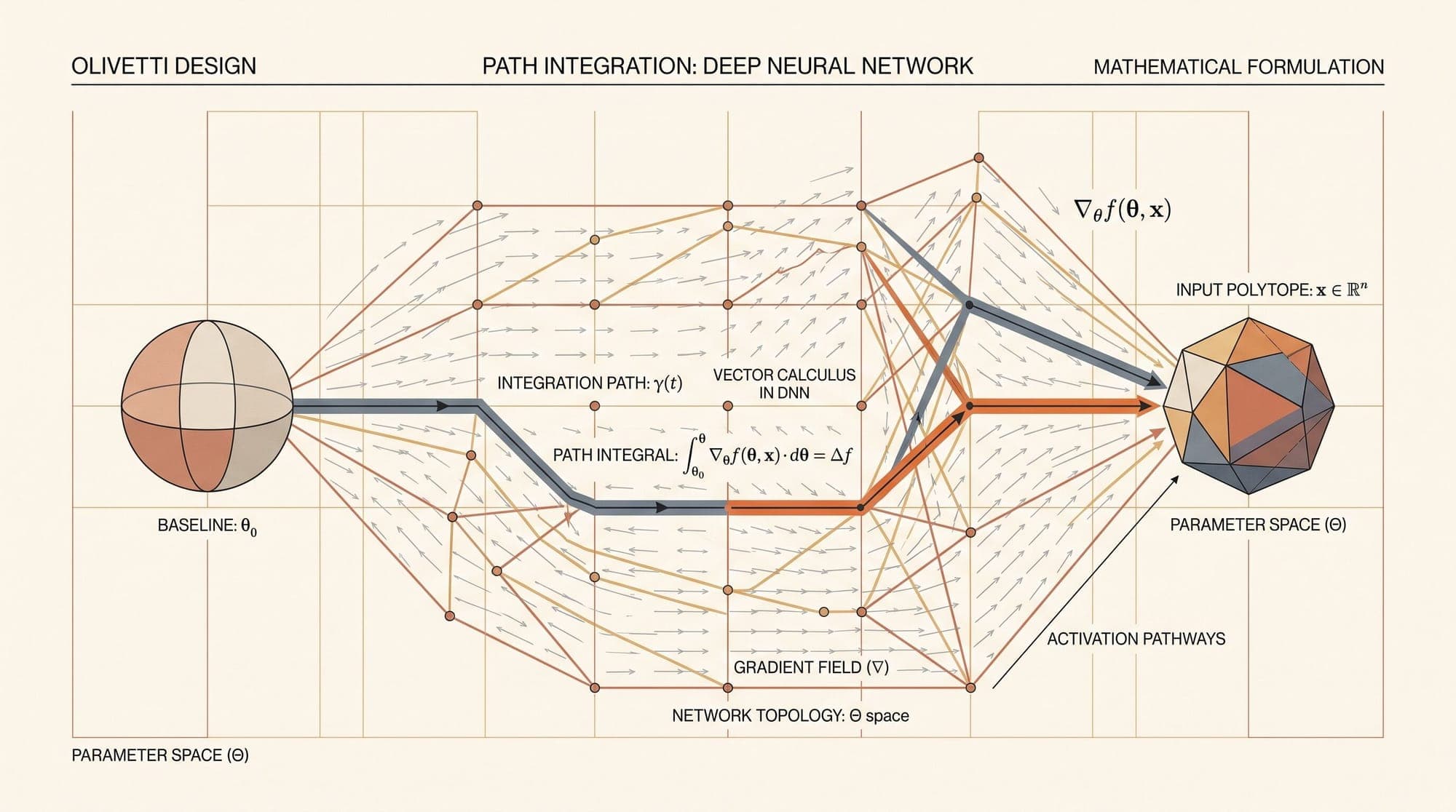
Integrated Gradients computes feature attribution by integrating the gradient of the model along the straight-line trajectory connecting the baseline $x'$ to the input $x$.

The Continuous Path Integral

Let $\gamma(\alpha)$ represent the straight-line path parameterized by $\alpha \in [0, 1]$:

$$\gamma(\alpha) = x' + \alpha (x - x')$$

The Integrated Gradient for the $i$-th feature dimension is defined as:

$$\text{IG}_i(x, x') = (x_i - x'_i) \times \int_{0}^{1} \frac{\partial F(x' + \alpha(x - x'))}{\partial x_i} \, d\alpha$$

Where $\frac{\partial F(z)}{\partial x_i}$ is the partial derivative of model $F$ along the $i$-th dimension evaluated at point $z$.

Proof of the Completeness Axiom

The mathematical property of Integrated Gradients lies in how directly it satisfies Completeness via the multivariate Fundamental Theorem of Calculus:

$$\sum_{i=1}^d \text{IG}_i(x, x') = \sum_{i=1}^d (x_i - x'_i) \int_0^1 \frac{\partial F(x' + \alpha(x - x'))}{\partial x_i} \, d\alpha$$

By swapping the summation and the integral:

$$\sum_{i=1}^d \text{IG}_i(x, x') = \int_0^1 \sum_{i=1}^d \frac{\partial F(\gamma(\alpha))}{\partial \gamma_i(\alpha)} \frac{d\gamma_i(\alpha)}{d\alpha} \, d\alpha$$

Applying the chain rule, the integrand is the total derivative of $F(\gamma(\alpha))$ with respect to $\alpha$:

$$\sum_{i=1}^d \text{IG}_i(x, x') = \int_0^1 \frac{d F(\gamma(\alpha))}{d\alpha} \, d\alpha = F(\gamma(1)) - F(\gamma(0)) = F(x) - F(x')$$

Because the line integral integrates through the entire transition from baseline to input, it captures gradients before, during, and after saturation points.

4. Numerical Approximation and Computational Architecture

Because neural networks are complex non-linear compositions, the integral cannot be evaluated in closed form. Instead, it is approximated numerically using discrete step summations.

Riemann Summation

The standard numerical approximation samples $m$ points uniformly along the straight line using Riemann summation:

$$\text{IG}_i^{\text{approx}}(x, x') = (x_i - x'_i) \times \frac{1}{m} \sum_{k=1}^m \frac{\partial F\left(x' + \frac{k}{m}(x - x')\right)}{\partial x_i}$$

Alternatively, Gauss-Legendre Quadrature can be used to select optimal evaluation nodes and weights, achieving higher integration accuracy with fewer function evaluations.

Baseline (x')                                                         Input (x)
  α = 0.0       α = 0.25        α = 0.50        α = 0.75        α = 1.0
    ○───────────────●───────────────●───────────────●───────────────●
  F(x')         ∇F(z_1)         ∇F(z_2)         ∇F(z_3)         F(x)

Convergence Monitoring and Step Calibration

To ensure the approximation is numerically sound, implementations compute the completeness error $\delta$:

$$\delta = \left| \sum_{i=1}^d \text{IG}_i^{\text{approx}}(x, x') - (F(x) - F(x')) \right|$$

In production auditing systems, the step count $m$ is typically set between $50$ and $300$. A step count is considered converged when the relative error $\frac{\delta}{|F(x) - F(x')|}$ falls below $5\%$.

Evaluating $m$ steps requires $m$ forward passes and $m$ backward passes per attribution run. When batching interpolation steps together ($[m \times d]$ tensors), GPU memory bandwidth becomes the primary performance bottleneck.

5. Applying Integrated Gradients to Transformers and Large Language Models

Applying Integrated Gradients to transformer-based language models introduces architectural challenges distinct from vision or tabular models.

Input Tokens:      ["The", "contract", "is", "void"]
                     │          │        │       │
Embedding Vectors: [ E_1  ,    E_2  ,   E_3  ,  E_4  ]  ∈ ℝ^(L × d_model)
                     │          │        │       │
               Interpolation along α ∈ [0, 1] against Baseline (e.g., [PAD] / 0)
                     │
               Layer Integrated Gradients (Capture dF / dE_j)
                     │
Vector IG:         [ IG_1 ,    IG_2 ,   IG_3 ,  IG_4 ]  ∈ ℝ^(L × d_model)
                     │          │        │       │
L2 Norm / Sum:     [ 0.04 ,    0.72 ,   0.08 ,  0.89 ]  → Scalar Token Attributions

1. Attributing Token Embeddings

In transformers, discrete token IDs cannot be directly differentiated. Integrated Gradients is instead computed with respect to the continuous token embedding vectors $E \in \mathbb{R}^{L \times d_{\text{model}}}$, where $L$ is sequence length and $d_{\text{model}}$ is hidden dimension.

For each token position $j$ and embedding dimension $k$:

$$\text{IG}_{j,k}(E, E') = (E_{j,k} - E'_{j,k}) \times \frac{1}{m} \sum_{s=1}^m \frac{\partial F\left(E' + \frac{s}{m}(E - E')\right)}{\partial E_{j,k}}$$

To convert the resulting $[L \times d_{\text{model}}]$ attribution matrix into a single scalar importance score per token, practitioners either sum across the embedding dimension or compute the Euclidean norm ($L_2$ norm):

$$\text{TokenScore}_j = \sum_{k=1}^{d_{\text{model}}} \text{IG}_{j,k} \quad \text{or} \quad \text{TokenScore}_j = \sqrt{\sum_{k=1}^{d_{\text{model}}} \left(\text{IG}_{j,k}\right)^2}$$

2. The NLP Baseline Selection Dilemma

The choice of baseline $x'$ represents the absence of information. In computer vision, a solid black or blurred image often serves as a natural baseline. In natural language, defining an empty text state is non-trivial, as explored by Sturmfels et al. (Distill 2020):

• Zero Embedding ($\mathbf{0}$): A vector of all zeros across the hidden dimension. Provides a simple, neutral mathematical reference point, but can produce out-of-distribution LayerNorm activations.
• Padding Token ([PAD]): The embedding vector of the tokenizer pad token. Models are explicitly trained to ignore pad tokens, though pad embeddings still retain non-zero positional and semantic weights.
• Mask Token ([MASK]): The embedding of the mask token in masked language models (BERT, RoBERTa). Represents unknown or hidden information, but is not natively present in causal autoregressive decoders.
• Average Embedding ($\bar{E}$): The mean embedding vector across the entire vocabulary. Represents the expected background language signal, though it blurs specific semantic contrasts.
• Empty String or Random Uniform: Embeddings of whitespace or random uniform draws. Tests input presence versus absence, though random initialization can introduce high-frequency noise.

Because changing the baseline changes the counterfactual question being asked ("why this prediction compared to what reference?"), the baseline must be chosen deliberately and reported alongside the attributions.

3. Layer Integrated Gradients

Beyond input embeddings, Layer Integrated Gradients evaluates attributions with respect to intermediate activations within specific transformer layers:

• Multi-Head Attention output projections
• Feed-Forward Network (FFN) intermediate activations
• Residual stream states at layer $l$

This enables interpretability researchers to trace how token representations evolve through the transformer stack, identifying exactly which layer resolves semantic ambiguities or retrieves factual knowledge.

6. Implementation with PyTorch and Captum

The PyTorch Captum library provides native support for Integrated Gradients and Layer Integrated Gradients. Below is an end-to-end implementation for attributing prediction probabilities to input token embeddings in a transformer model:

import torch
from captum.attr import IntegratedGradients, LayerIntegratedGradients

class TransformerExplainer:
    def __init__(self, model, tokenizer):
        self.model = model
        self.tokenizer = tokenizer
        self.model.eval()
        
        # Initialize Layer Integrated Gradients targeting word embeddings
        self.lig = LayerIntegratedGradients(
            self._forward_wrapper, 
            self.model.transformer.wte
        )

    def _forward_wrapper(self, input_embeddings, attention_mask=None):
        # Forward pass consuming continuous embedding tensors
        outputs = self.model(inputs_embeds=input_embeddings, attention_mask=attention_mask)
        # Return target class logit or target token probability
        return outputs.logits[:, -1, :]

    def explain(self, text, target_token_id, n_steps=100):
        # 1. Encode text
        inputs = self.tokenizer(text, return_tensors="pt")
        input_ids = inputs["input_ids"]
        attention_mask = inputs["attention_mask"]

        # 2. Build baseline: all [PAD] tokens (or zero token IDs)
        pad_id = self.tokenizer.pad_token_id or 0
        baseline_ids = torch.full_like(input_ids, fill_value=pad_id)

        # 3. Compute Layer Integrated Gradients
        # Returns attributions with shape [batch, seq_len, hidden_dim]
        attributions, delta = self.lig.attribute(
            inputs=input_ids,
            baselines=baseline_ids,
            target=target_token_id,
            additional_forward_args=(attention_mask,),
            n_steps=n_steps,
            return_convergence_delta=True
        )

        # 4. Collapse hidden dimension into scalar token scores
        token_attributions = attributions.sum(dim=-1).squeeze(0)
        
        # Normalize scores for visualization
        token_attributions = token_attributions / torch.norm(token_attributions)
        tokens = self.tokenizer.convert_ids_to_tokens(input_ids.squeeze(0))

        return list(zip(tokens, token_attributions.detach().cpu().numpy())), delta.item()

7. Extensions, Manifold Paths, and Limitations

While Integrated Gradients is mathematically rigorous and uniquely axiomatic among straight-line path methods, practical deployments must account for several structural limitations:

Out-of-Distribution Interpolation

The straight line $\gamma(\alpha) = x' + \alpha(x - x')$ in high-dimensional embedding space frequently travels through non-manifold regions (combinations of token features that would never naturally occur in pre-training data). Gradients evaluated in these unrealistic spaces can introduce noise into the attribution sum.

To counter this, advanced path variants have been developed:

• Guided Integrated Gradients (GIG): Adapts the integration path step-by-step to avoid high-gradient saturated ridges.
• Blur Integrated Gradients (Blur IG): For image models, sweeps spatial frequencies from blurred baselines rather than linear pixel interpolation.
• Expected Gradients (IG with Prior Distributions): Averages straight-line paths across an empirical distribution of baselines $x' \sim \mathcal{D}_{\text{baseline}}$, softening reliance on a single reference vector.

Computational Overhead

Unlike single-pass saliency or attention-weight heuristics, Integrated Gradients requires dozens to hundreds of backward passes per instance. In production RAG monitoring or real-time guardrail systems, running full IG passes on every request is computationally prohibitive. Teams typically run Integrated Gradients asynchronously for root-cause debugging, safety auditing, model evaluation, and offline red-teaming.

Summary

Integrated Gradients bridges continuous vector calculus and axiomatic game theory to solve the gradient saturation bottleneck in deep neural network interpretability. By integrating gradients along the straight-line trajectory between a neutral baseline and the target input:

• It guarantees Completeness ($F(x) - F(x') = \sum \text{IG}_i$).
• It preserves Implementation Invariance across functionally equivalent architectures.
• It restores Sensitivity, capturing the cumulative contribution of features even when local derivatives have flattened to zero.

For transformer models and LLMs, Integrated Gradients provides a principled, ground-truth attribution mechanism for token embeddings, attention modules, and intermediate residual streams, moving model interpretability beyond superficial attention heatmaps into mathematically grounded causal attribution.

Sources

• Sundararajan, Mukund, Ankur Taly, and Qiqi Yan. "Axiomatic Attribution for Deep Networks." Proceedings of the 34th International Conference on Machine Learning (ICML), PMLR 70:3319-3328, 2017.
• Aumann, Robert J., and Lloyd S. Shapley. "Values of Non-Atomic Games." Princeton University Press, 1974.
• Friedman, Eric. "Paths to compromise in economic design." Journal of Mathematical Economics, 40(3-4):257-278, 2004.
• Mudrakarta, Pramod Kaushik, et al. "Did the Model Understand the Question?" Proceedings of the 56th Annual Meeting of the Association for Computational Linguistics (ACL), 2018.
• Sturmfels, Pascal, et al. "Visualizing the Impact of Feature Attribution Baselines." Distill, 2020.
• Shrikumar, Avanti, Peyton Greenside, and Anshul Kundaje. "Learning Important Features Through Propagating Activation Differences." Proceedings of the 34th International Conference on Machine Learning (ICML), 2017.
• Kokhlikyan, Narine, et al. "Captum: A unified and generic model interpretability library for PyTorch." arXiv preprint arXiv:2009.07896, 2020.