Grouped-Query Attention and Multi-Query Attention: Mathematical Foundations, KV Cache Bandwidth Scaling, and Inference Economics

Autoregressive generation in Large Language Models presents an asymmetric computational profile. During prompt processing (prefill), computation is compute-bound, executing large matrix multiplications that fully saturate modern Tensor Cores. During token-by-token generation (decoding), execution shifts entirely to a memory-bandwidth-bound regime. Each newly generated token requires fetching all prior Key and Value (KV) activation tensors from High Bandwidth Memory (HBM) to on-chip SRAM to compute attention weights, while performing only a single vector-matrix product.

Standard Multi-Head Attention (MHA) creates independent Key and Value projections for every Query head. At long context lengths and large batch sizes, the resulting KV cache footprint consumes tens of gigabytes of GPU memory and saturates memory bus bandwidth, capping serving throughput.

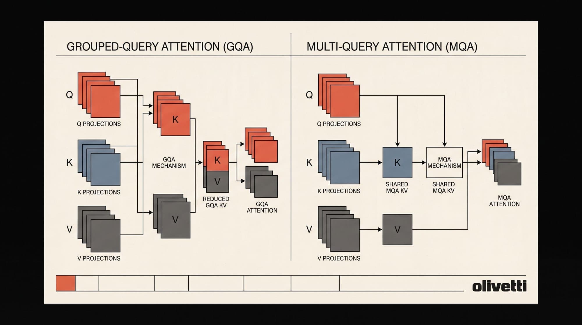
To break this memory wall, Shazeer (2019) introduced Multi-Query Attention (MQA), collapsing all Key and Value heads into a single shared projection. While MQA dramatically reduces memory traffic, it induces capacity loss on complex reasoning and long-context retrieval tasks. Ainslie et al. (2023) resolved this trade-off with Grouped-Query Attention (GQA), partitioning Query heads into distinct subgroups that share Key and Value projections.

Today, GQA has become the standard attention mechanism across modern open-weight and proprietary architectures, including LLaMA 3 (Meta, 2024), Mistral 7B (Jiang et al., 2023), and Gemma 2 (Google, 2024).

The Arithmetic Intensity Wall in Autoregressive Serving

The computational efficiency of deep learning kernels on hardware accelerators is governed by the Roofline Model, defined by arithmetic intensity:

Arithmetic Intensity = Total Floating-Point Operations (FLOPs) / Total Memory Transferred (Bytes)

On an NVIDIA H100 SXM5 GPU, peak FP16/BF16 Tensor Core throughput is 989 TFLOPs/s, while peak HBM3 memory bandwidth is 3.35 TB/s. The hardware operational ceiling requires an arithmetic intensity of at least:

Critical Intensity = (989 * 10^12 FLOPs/s) / (3.35 * 10^12 Bytes/s) ≈ 295 FLOPs / Byte

Any operation with an arithmetic intensity below 295 FLOPs/Byte is memory-bandwidth bound, meaning the execution speed is strictly constrained by how fast bytes move across the memory bus, leaving compute cores idle.

During autoregressive generation of a single token with batch size b=1, the model reads the entire KV cache history of length s across L layers with hidden dimension d_model. For a single attention layer, reading the KV cache requires transferring:

Memory Traffic_KV = 2 * b * s * d_model * sizeof(dtype) Bytes

The floating-point computation required to compute attention over s historical tokens is:

Compute_Attention = 4 * b * s * d_model FLOPs

Computing the arithmetic intensity of the attention kernel during single-token decoding (using 16-bit precision, sizeof(dtype) = 2):

Arithmetic Intensity_Decode = (4 * b * s * d_model) / (4 * b * s * d_model) = 1 FLOP / Byte

An arithmetic intensity of 1 FLOP/Byte is more than two orders of magnitude below the saturation point of the processor. Consequently, the time required to generate each token in autoregressive decoding is directly proportional to the total bytes read from the KV cache.

Mathematical Formulations: MHA, MQA, and GQA

Let x ∈ R^(b * s * d_model) represent the input activation tensor to a Transformer layer. Let H denote the total number of Query attention heads, and let d_k = d_v = d_head = d_model / H denote the head dimension.

1. Multi-Head Attention (MHA)

In standard Multi-Head Attention as formulated by Vaswani et al. (2017), the layer instantiates H independent Query, Key, and Value projection matrices:

W_Q ∈ R^(d_model * (H * d_head)) W_K ∈ R^(d_model * (H * d_head)) W_V ∈ R^(d_model * (H * d_head))

For each head i ∈ {1, ..., H}:

Q_i = x * W_Q^(i) ∈ R^(b * s * d_head) K_i = x * W_K^(i) ∈ R^(b * s * d_head) V_i = x * W_V^(i) ∈ R^(b * s * d_head)

Head_i = Softmax( (Q_i * (K_i)^T) / sqrt(d_head) ) * V_i ∈ R^(b * s * d_head)

MHA(x) = Concat(Head_1, ..., Head_H) * W_O

In MHA, the number of Key heads H_K and Value heads H_V equals the number of Query heads: H_Q = H_K = H_V = H.

2. Multi-Query Attention (MQA)

Multi-Query Attention (Shazeer, 2019) eliminates independent Key and Value projections per head. While keeping H independent Query heads, MQA collapses Key and Value projections to a single shared head (H_K = H_V = 1):

W_Q ∈ R^(d_model * (H * d_head)) W_K ∈ R^(d_model * d_head) W_V ∈ R^(d_model * d_head)

The shared Key and Value tensors K, V ∈ R^(b * s * d_head) are broadcast across all H Query heads:

For i ∈ {1, ..., H}: Head_i = Softmax( (Q_i * K^T) / sqrt(d_head) ) * V

MQA(x) = Concat(Head_1, ..., Head_H) * W_O

MQA reduces the parameter footprint of W_K and W_V by a factor of H, and cuts the KV cache memory size and memory traffic by an exact factor of H.

3. Grouped-Query Attention (GQA)

Grouped-Query Attention (Ainslie et al., 2023) provides a generalized mathematical interpolation between MHA and MQA.

The H Query heads are partitioned into G distinct groups, where each group contains M = H / G Query heads. Each group shares a single Key head and a single Value head (H_K = H_V = G):

W_Q ∈ R^(d_model * (H * d_head)) W_K ∈ R^(d_model * (G * d_head)) W_V ∈ R^(d_model * (G * d_head))

Let g ∈ {1, ..., G} index the group, and let m ∈ {1, ..., M} index the query head within group g. The Query head index is i = (g - 1) * M + m.

For each group g: K_g = x * W_K^(g) ∈ R^(b * s * d_head) V_g = x * W_V^(g) ∈ R^(b * s * d_head)

For each Query head i belonging to group g: Q_i = x * W_Q^(i) ∈ R^(b * s * d_head) Head_i = Softmax( (Q_i * (K_g)^T) / sqrt(d_head) ) * V_g

GQA(x) = Concat(Head_1, ..., Head_H) * W_O

Special cases:

When G = H (group size M = 1), GQA is identical to Multi-Head Attention (MHA).
When G = 1 (group size M = H), GQA is identical to Multi-Query Attention (MQA).

Architectural comparison of MHA, GQA, and MQA head groupings

Quantitative KV Cache Footprint and Bandwidth Economics

The total memory footprint of the KV cache across a model with L layers, sequence length s, batch size b, and head dimension d_head is:

Memory_KV = 2 * b * s * L * H_KV * d_head * sizeof(dtype) Bytes

Where H_KV is the number of Key-Value heads (H for MHA, 1 for MQA, and G for GQA).

Consider a 70-billion parameter model architecture (such as LLaMA 2 or LLaMA 3) with parameters:

Layers L = 80
Hidden dimension d_model = 8192
Query heads H = 64, Head dimension d_head = 128
Precision: 16-bit float (sizeof(dtype) = 2 bytes)
Sequence length s = 8192 tokens
Batch size b = 16

Let us evaluate the memory consumption and bandwidth requirements across the three architectures:

Case 1: Multi-Head Attention (MHA, H_KV = 64)

KV Cache Size = 2 * 16 * 8192 * 80 * 64 * 128 * 2 Bytes
KV Cache Size = 343.60 GB
At batch size 16 and context length 8k, the KV cache exceeds the physical VRAM capacity of four 80GB GPUs combined.

Case 2: Grouped-Query Attention (GQA-8, G = 8, M = 8)

KV Cache Size = 2 * 16 * 8192 * 80 * 8 * 128 * 2 Bytes
KV Cache Size = 42.95 GB
Reduction Factor: 8x reduction compared to MHA. Fits comfortably within a single 80GB GPU.

Case 3: Multi-Query Attention (MQA, G = 1)

KV Cache Size = 2 * 16 * 8192 * 80 * 1 * 128 * 2 Bytes
KV Cache Size = 5.37 GB
Reduction Factor: 64x reduction compared to MHA.

Serving Throughput Impact

Because token generation latency is constrained by memory transfer time (Latency_step ≈ Memory_KV / Bandwidth_HBM), reducing KV cache size by 8x through GQA directly reduces the memory traffic per forward step by 8x.

For a serving system configured with Tensor Parallelism (TP=8), GQA allows increasing the serving batch size by 8x at identical memory footprint, leading to near-linear increases in token generation throughput (tokens/second/GPU).

Checkpoint Uptraining and Mean-Pooling Conversion

Training frontier foundation models from scratch requires millions of GPU hours. Ainslie et al. (2023) established an efficient method for converting existing pre-trained MHA model checkpoints into GQA models via Mean-Pooling Initialization followed by a brief uptraining stage.

1. Weight Mean-Pooling

Given a pre-trained MHA checkpoint with H Key and Value projection matrices {W_K^(1), ..., W_K^(H)} and {W_V^(1), ..., W_V^(H)}, the G Grouped-Query projections are initialized by computing the arithmetic mean over the M = H / G projection matrices within each group g:

W_K^(g) = (1 / M) * \sum_{m=1}^M W_K^((g - 1) * M + m)

W_V^(g) = (1 / M) * \sum_{m=1}^M W_V^((g - 1) * M + m)

The Query projection weights W_Q and Output projection weights W_O are transferred directly from the MHA checkpoint without modification.

2. Uptraining Dynamics

After mean-pooling initialization, the model experiences an initial spike in cross-entropy loss due to the loss of per-head key-value subspace diversity. However, because W_Q and W_O retain their trained representations, the model rapidly recovers full representational accuracy within a small fraction of original pre-training compute.

Empirical results demonstrated that uptraining a converted GQA checkpoint on just 5% of the original pre-training token budget fully matched the perplexity and downstream evaluation scores of the original dense MHA baseline across summarization, question answering, and multi-turn reasoning tasks.

Representational Capacity and Empirical Trade-Offs

Why does GQA outperform MQA while capturing nearly the full memory savings?

In standard Multi-Head Attention, each query head computes attention over an independent subspace of key-value representations:

Subspace_i = { (K_i * x, V_i * x) | x ∈ R^(d_model) }

This allows head i to track syntactic relations (e.g. subject-verb agreement) while head j tracks semantic coreference or positional induction patterns.

In MQA, all H query heads are forced to attend over a single, identical key-value subspace:

Subspace_MQA = { (K * x, V * x) }

Although each query head can compute distinct dot-product scores Q_i * K^T, the values being retrieved and mixed are constrained to a single subspace. On long-context tasks (such as document retrieval or Needle-in-a-Haystack tests) and multi-step mathematical reasoning, MQA suffers measurable degradation because the single value projection cannot preserve sufficient token diversity.

GQA restores subspace capacity by maintaining G independent key-value subspaces. Empirical ablations from Ainslie et al. (2023) and Touvron et al. (2023) demonstrated that setting G = 8 (with H = 32 or H = 64) achieves:

Accuracy: Zero statistically significant degradation compared to full MHA across MMLU, GSM8K, HumanEval, and SQuAD.
Memory: 75% to 87.5% reduction in KV cache memory consumption.
Inference Speed: 3x to 6x speedup in autoregressive decoding latency under high batch concurrency.

Distributed Systems and Tensor Parallelism Constraints

In distributed LLM serving frameworks (such as Megatron-LM, vLLM, and TensorRT-LLM), model weights are partitioned across multiple GPUs using Tensor Parallelism (TP).

In standard Column Parallel Linear layers, projection weights are partitioned along their output dimension:

Query projections are partitioned into H / TP heads per GPU.
Key and Value projections are partitioned into G / TP heads per GPU.

This introduces a fundamental hardware constraint for GQA:

G mod TP = 0

The number of Key-Value groups G must be an integer multiple of the Tensor Parallelism degree TP.

For example:

In LLaMA 3 70B (H = 64, G = 8), the model can be natively sharded across TP = 1, 2, 4, or 8 GPUs without cross-device communication for KV heads.
If a deployment requires TP = 16, each KV head would have to be replicated or split along the hidden dimension (d_head), introducing additional communication collectives or unbalanced memory layouts.

Modern serving runtimes combine GQA with PagedAttention (Kwon et al., 2023) and FlashDecoding (Dao et al., 2023), which partition the sequence dimension across streaming multiprocessors during decoding to further accelerate GQA kernels.

Summary of Architectural Specifications

The progression of attention architectures across modern foundation models highlights the transition to GQA:

Vaswani Transformer / LLaMA 1 / LLaMA 2 (7B, 13B): Multi-Head Attention (MHA). H_Q = 32, H_KV = 32. Maximum representational capacity, high KV cache memory overhead.
Falcon (7B, 40B) / StarCoder 1: Multi-Query Attention (MQA). H_Q = 64 / 128, H_KV = 1. Maximum memory reduction, potential degradation on complex multi-hop retrieval.
LLaMA 2 70B / LLaMA 3 (8B, 70B, 405B): Grouped-Query Attention (GQA). H_Q = 32 / 64 / 128, H_KV = 8. 4x to 16x KV cache reduction, zero measurable accuracy loss.
Mistral 7B / Mixtral 8x7B: Grouped-Query Attention (GQA). H_Q = 32, H_KV = 8. Combined with Sliding Window Attention for efficient local context caching.
Gemma 2 (9B, 27B): Grouped-Query Attention (GQA). H_Q = 16 / 32, H_KV = 8 / 16. Combined with alternating local and global attention layers.