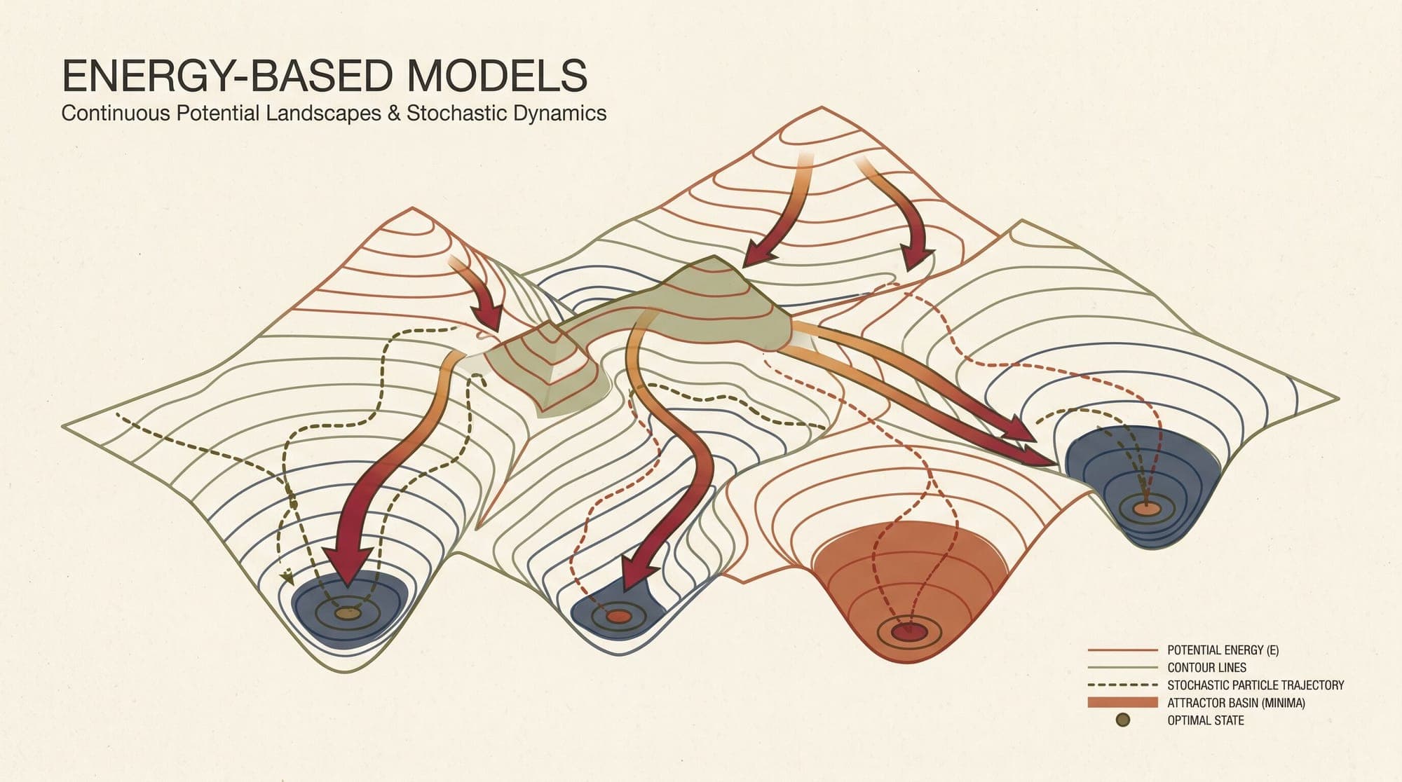
Energy-Based Models: How Energy Landscapes, Contrastive Divergence, and Langevin Dynamics Unify Generative Learning

Probabilistic modeling in machine learning fundamentally centers on estimating data distributions over high-dimensional spaces. Standard generative architectures achieve this by enforcing structural constraints: autoregressive models factorize joint distributions through causal chains, normalizing flows constrain network architectures to invertible bijections with tractable Jacobian determinants, variational autoencoders optimize surrogate lower bounds over latent spaces, and generative adversarial networks bypass density estimation through two-player minimax games.

Energy-Based Models (EBMs) eliminate these architectural constraints. An EBM maps any arbitrary input configuration to a single unconstrained real scalar value termed its energy. By assigning low energy values to plausible data points and high energy values to implausible or corrupt configurations, EBMs define flexible probability densities that underpin modern score-based diffusion, modern Hopfield networks, self-supervised representation learning, and preference alignment algorithms.

The Boltzmann-Gibbs Formulation and the Intractable Partition Function

Formally, an energy-based model defines the probability density $p_\theta(x)$ over a continuous domain $\mathcal{X} \subseteq \mathbb{R}^D$ using a parameterized neural network $E_\theta(x): \mathbb{R}^D \to \mathbb{R}$:

$$p_\theta(x) = \frac{\exp(-E_\theta(x))}{Z(\theta)}$$

The normalizing factor $Z(\theta)$, known as the partition function in statistical physics, integrates the unnormalized Boltzmann factor over the entire input space:

$$Z(\theta) = \int_{\mathcal{X}} \exp(-E_\theta(x)) \, dx$$

Because the partition function requires integration over high-dimensional continuous domains, exact computation of $Z(\theta)$ is analytically and computationally intractable for non-trivial neural energy functions.

When training an EBM via maximum likelihood estimation on an empirical dataset $\mathcal{D} = \{x_1, \dots, x_N\}$, the objective minimizes the negative log-likelihood loss:

$$\mathcal{L}(\theta) = -\frac{1}{N} \sum_{i=1}^N \log p_\theta(x_i) = \frac{1}{N} \sum_{i=1}^N E_\theta(x_i) + \log Z(\theta)$$

Taking the gradient of the log-likelihood with respect to model parameters $\theta$ yields:

$$\nabla_\theta \log p_\theta(x) = -\nabla_\theta E_\theta(x) - \nabla_\theta \log Z(\theta)$$

Evaluating the gradient of the log-partition function reveals a fundamental identity:

$$\nabla_\theta \log Z(\theta) = \frac{1}{Z(\theta)} \nabla_\theta \int_{\mathcal{X}} \exp(-E_\theta(x)) \, dx = \int_{\mathcal{X}} \frac{\exp(-E_\theta(x))}{Z(\theta)} \left(-\nabla_\theta E_\theta(x)\right) dx = -\mathbb{E}_{x^- \sim p_\theta(x)}[\nabla_\theta E_\theta(x^-)]$$

Substituting this identity back into the log-likelihood gradient reveals the dual-phase learning dynamic that governs all energy-based training:

$$\nabla_\theta \log p_\theta(x) = \underbrace{-\nabla_\theta E_\theta(x_{\text{data}})}_{\text{Positive Phase (Pulls Down Data Energy)}} + \underbrace{\mathbb{E}_{x^- \sim p_\theta(x)}[\nabla_\theta E_\theta(x^-)]}_{\text{Negative Phase (Pushes Up Hallucination Energy)}}$$

In the positive phase, the optimizer adjusts parameters to decrease the energy assigned to observed training samples $x_{\text{data}}$. In the negative phase, the optimizer increases the energy of negative samples $x^-$ drawn from the model's current predictive distribution $p_\theta(x)$. Without the negative phase, the energy function suffers collapse, assigning uniform zero energy across all inputs.

Sampling from Energy Landscapes: Langevin Dynamics

Because $p_\theta(x)$ is unnormalized and lacks ancestral factorization, standard forward sampling cannot generate synthetic samples in a single pass. Instead, sampling relies on Markov Chain Monte Carlo (MCMC) algorithms, primarily Stochastic Gradient Langevin Dynamics (SGLD) introduced by Welling and Teh (2011).

Langevin dynamics simulates Brownian motion across the continuous potential landscape defined by $E_\theta(x)$. Given an initial sample $x_0$ drawn from a broad prior distribution (such as uniform noise $\mathcal{U}[-1, 1]^D$), the chain updates iteratively over discrete time steps $t$:

$$x_{t+1} = x_t - \frac{\epsilon}{2} \nabla_x E_\theta(x_t) + \sqrt{\epsilon} z_t, \quad z_t \sim \mathcal{N}(0, I)$$

Here, $\epsilon > 0$ represents the step size, $\nabla_x E_\theta(x_t)$ is the spatial gradient of the energy function evaluated with respect to the input, and $z_t$ is standard isotropic Gaussian noise.

The update consists of two opposing forces:

1. Deterministic Drift ($-\frac{\epsilon}{2} \nabla_x E_\theta(x_t)$): Guides the state vector down the steepest energy descent path toward high-probability attractor basins.
2. Stochastic Diffusion ($\sqrt{\epsilon} z_t$): Injects Brownian fluctuations to prevent the trajectory from getting trapped in shallow local minima and ensures exploration of the full probability density.

As the step size $\epsilon \to 0$ and the number of steps $t \to \infty$, the distribution of samples generated by this Langevin diffusion process converges asymptotically to the exact model distribution $p_\theta(x)$.

To scale Langevin sampling to high-dimensional continuous domains like images, Du and Mordatch (2019) introduced key stability mechanisms:

• Persistent Replay Buffers: Instead of initializing Langevin chains from pure noise at every training iteration, negative samples are initialized from a historical replay buffer with high probability (e.g., 95%) and from random noise with low probability (5%). This allows MCMC chains to maintain persistent trajectories across training iterations.
• Gradient Clipping: Clamping $\nabla_x E_\theta(x)$ prevents exploding gradient steps caused by steep energy cliffs.
• Langevin Step Schedules: Running 40 to 100 Langevin steps with decaying step sizes per training step provides stable convergence on complex benchmarks.

Training EBMs: Contrastive Divergence and Score Matching

Running MCMC chains to full asymptotic equilibrium at every training step is computationally prohibitive. Several mathematical frameworks bypass full equilibrium sampling:

Contrastive Divergence ($CD_k$)

Introduced by Hinton (2002), Contrastive Divergence replaces full stationary MCMC sampling with short, non-converged Markov chains. Rather than initializing from random noise, $CD_k$ initializes the Markov chain directly at the empirical data point $x^{(0)} = x_{\text{data}}$ and executes only $k$ steps of Gibbs or Langevin transitions:

$$x^{(0)} \sim p_{\text{data}} \xrightarrow{k \text{ steps}} x^{(k)}$$

The parameter update approximates the true log-likelihood gradient using this truncated sample:

$$\Delta \theta \approx -\nabla_\theta E_\theta(x^{(0)}) + \nabla_\theta E_\theta(x^{(k)})$$

Even with $k=1$, $CD_1$ provides an effective, though slightly biased, optimization direction that pulls down data energy while lifting energy in the immediate local neighborhood of observed data.

Score Matching and Denoising Score Matching

Instead of estimating the unnormalized density $p_\theta(x)$, Hyvärinen (2005) proposed matching the score function, defined as the spatial gradient of the log-density with respect to input $x$:

$$s_\theta(x) = \nabla_x \log p_\theta(x) = -\nabla_x E_\theta(x) - \underbrace{\nabla_x \log Z(\theta)}_{= 0} = -\nabla_x E_\theta(x)$$

Because the partition function $Z(\theta)$ depends only on parameters $\theta$ and does not vary with input $x$, its spatial derivative $\nabla_x \log Z(\theta)$ is identically zero. The score function is independent of the partition function.

Explicit score matching minimizes the expected squared error between the model score and the true data score:

$$\mathcal{J}_{\text{ESM}}(\theta) = \frac{1}{2} \mathbb{E}_{x \sim p_{\text{data}}}\left[\|\nabla_x \log p_\theta(x) - \nabla_x \log p_{\text{data}}(x)\|^2\right]$$

Using integration by parts, Hyvärinen eliminated the unobservable ground-truth score $\nabla_x \log p_{\text{data}}(x)$, rewriting the objective as:

$$\mathcal{J}_{\text{SM}}(\theta) = \mathbb{E}_{x \sim p_{\text{data}}}\left[\text{Tr}(\nabla_x^2 \log p_\theta(x)) + \frac{1}{2} \|\nabla_x \log p_\theta(x)\|^2\right]$$

To eliminate the expensive computation of the Hessian trace $\text{Tr}(\nabla_x^2 \log p_\theta(x))$, Vincent (2011) developed Denoising Score Matching (DSM). By corrupting inputs with known Gaussian noise $q_\sigma(\tilde{x}|x) = \mathcal{N}(\tilde{x}; x, \sigma^2 I)$, the analytical score of the perturbation kernel $\nabla_{\tilde{x}} \log q_\sigma(\tilde{x}|x) = -\frac{\tilde{x} - x}{\sigma^2}$ is known, yielding the simplified objective:

$$\mathcal{L}_{\text{DSM}}(\theta) = \mathbb{E}_{x \sim p_{\text{data}}, \tilde{x} \sim q_\sigma(\tilde{x}|x)}\left[\left\|s_\theta(\tilde{x}) + \frac{\tilde{x} - x}{\sigma^2}\right\|^2\right]$$

The Unifying Bridge to Modern Generative AI and LLMs

Energy-based formulations serve as the underlying mathematical scaffolding across several distinct domains in modern artificial intelligence:

1. Score-Based Diffusion Models

In a landmark synthesis, Song and Ermon (2019) connected score matching on energy landscapes to generative diffusion models. A score-based diffusion model trains a noise-conditional neural network $s_\theta(x, \sigma)$ to predict energy gradients across a geometric ladder of perturbation scales $\sigma_1 < \sigma_2 < \dots < \sigma_L$.

Sampling then executes Annealed Langevin Dynamics, initiating MCMC at the highest noise scale $\sigma_L$ where the energy landscape is smooth and unimodal, and gradually decreasing the noise level toward $\sigma_1$. This resolves the classic mode-mixing failure of standard EBMs by smoothing out steep energy barriers at initial generation stages.

2. Joint Energy-Based Models (JEM)

Grathwohl et al. (2019) proved that any standard discriminative neural network classifier is secretly an energy-based model. For a classifier parameterized by $f_\theta(x): \mathbb{R}^D \to \mathbb{R}^K$ producing logits for $K$ discrete classes, the joint probability over inputs and classes is defined as:

$$p_\theta(x, y) = \frac{\exp(f_\theta(x)[y])}{Z(\theta)}$$

Marginalizing over all class labels $y$ reveals the implicit marginal distribution of input $x$:

$$p_\theta(x) = \sum_{y=1}^K p_\theta(x, y) = \frac{\sum_{y=1}^K \exp(f_\theta(x)[y])}{Z(\theta)} = \frac{\exp\left(\text{LogSumExp}_y(f_\theta(x)[y])\right)}{Z(\theta)}$$

This defines an unnormalized energy function directly from classifier logits:

$$E_\theta(x) = -\text{LogSumExp}_y(f_\theta(x)[y])$$

By training this objective with a hybrid loss combining standard cross-entropy classification and Langevin-based contrastive divergence, a single model performs competitive classification, state-of-the-art out-of-distribution detection, and unconditional generative synthesis simultaneously.

3. Modern Continuous Hopfield Networks

Ramsauer et al. (2020) demonstrated that the self-attention mechanism in Transformer architectures is mathematically equivalent to the state update rule of a modern continuous Hopfield network. The energy function governing stored memory patterns $\{x_1, \dots, x_N\}$ and state vector $\xi$ is given by:

$$E(\xi) = -\text{lse}\left(\beta, X^T \xi\right) + \frac{1}{2} \|\xi\|^2 + C$$

Applying concave-convex procedure minimization to this energy function yields the exact scaled dot-product softmax attention formula:

$$\xi^{\text{new}} = X \, \text{softmax}\left(\beta X^T \xi\right)$$

Transformers can thus be understood as dynamical systems performing energy minimization over associative memory representations.

4. Preference Alignment in Large Language Models

The energy-based formulation also underpins modern reinforcement learning from human feedback. In Direct Preference Optimization (DPO), the Bradley-Terry preference probability for a preferred completion $y_w$ over a dispreferred completion $y_l$ given prompt $x$ is defined as:

$$p(y_w \succ y_l | x) = \sigma\left(r(x, y_w) - r(x, y_l)\right)$$

Under optimal policy derivations, the scalar reward $r(x, y)$ corresponds directly to the negative energy of the completion under the fine-tuned model relative to a frozen reference model:

$$r(x, y) = \beta \log \frac{\pi_\theta(y|x)}{\pi_{\text{ref}}(y|x)} \equiv -E_\theta(y; x)$$

DPO optimizes an energy landscape where preferred tokens have their energy decreased (likelihood increased) and dispreferred tokens have their energy increased (likelihood decreased), exactly mirroring the positive and negative phases of contrastive divergence.

Architectural Trade-Offs and System Characteristics

| Dimension | Energy-Based Models (EBM) | Diffusion / Score Models | Autoregressive Transformers | Flow Matching | | :--- | :--- | :--- | :--- | :--- | | Density Evaluation | Unnormalized ($E_\theta(x)$ only; $Z$ intractable) | Approximate lower bound via SDE integration | Exact normalized likelihood via causal chain rule | Exact normalized likelihood via Continuous Normalizing Flows | | Sampling Mechanism | Iterative MCMC / Langevin dynamics | Iterative reverse SDE/ODE solvers | Step-by-step causal token generation | Numerical ODE integration (Euler / RK4) | | Architectural Restrictions | Completely unconstrained ($f(x) \to \mathbb{R}$) | Must output vector equal to input dimension | Causal autoregressive masking required | Vector field regressor ($v_t(x) \in \mathbb{R}^D$) | | Training Stability | Moderate to challenging (MCMC divergence risk) | High (stable score matching loss) | High (convex cross-entropy per step) | High (direct regression objective) | | Inference Latency | High (tens to hundreds of gradient steps) | High to moderate (10-50 ODE steps) | Proportional to sequence length ($O(N)$ forward passes) | Low to moderate (10-30 ODE integration steps) |

Core Failure Modes in High-Dimensional Energy Landscapes

1. Metastable States and Slow MCMC Mixing: In high-dimensional spaces with complex data distributions, probability mass clusters in isolated modes separated by massive energy barriers. Standard Langevin dynamics requires exponential time to cross these barriers, causing negative sampling chains to over-sample local modes while missing others.
2. Out-of-Distribution Energy Overestimation: Without explicit regularization or negative sampling across the entire input domain, neural energy functions frequently assign uncharacteristically low energy to bizarre, non-natural inputs lying far outside the training distribution manifold.
3. Training Instability: If the Langevin step size $\epsilon$ or gradient norm grows too large during negative phase sampling, MCMC chains can diverge into numerical overflow, destabilizing the entire parameter optimization process.

Summary

Energy-Based Models provide a mathematically unified perspective on probabilistic learning. By discarding the requirement that neural outputs integrate to unity, EBMs decouple representation architectures from density normalization. While training unnormalized models requires navigating the intractable partition function via contrastive divergence, score matching, or Langevin dynamics, the resulting energy principles directly inform score-based diffusion, attention dynamics, associative memories, and alignment objectives across modern artificial intelligence.

Sources

• A Tutorial on Energy-Based Learning (LeCun et al., 2006)
• Training Products of Experts by Minimizing Contrastive Divergence (Hinton, 2002)
• Bayesian Learning via Stochastic Gradient Langevin Dynamics (Welling and Teh, 2011)
• Estimation of Non-Normalized Statistical Models by Score Matching (Hyvärinen, 2005)
• A Connection Between Score Matching and Denoising Autoencoders (Vincent, 2011)
• Implicit Generation and Modeling with Energy Based Models (Du and Mordatch, 2019)
• Generative Modeling by Estimating Gradients of the Data Distribution (Song and Ermon, 2019)
• Your Classifier is Secretly an Energy Based Model and You Should Treat It Like One (Grathwohl et al., 2019)
• Hopfield Networks is All You Need (Ramsauer et al., 2020)
• Direct Preference Optimization: Your Language Model is Secretly a Reward Model (Rafailov et al., 2023)