Centered Kernel Alignment: How CKA Measures Representation Similarity Across Layers and Architectures

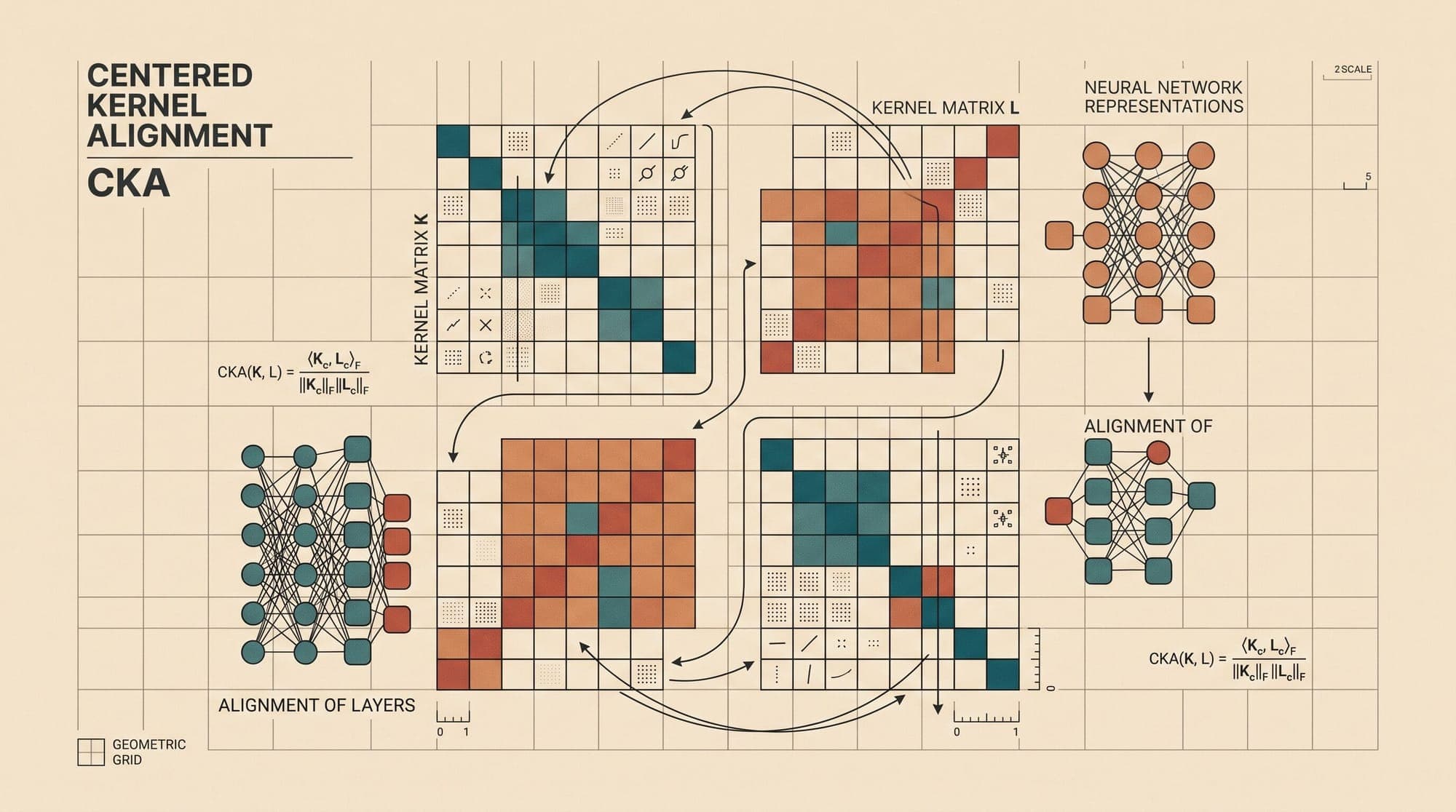
Understanding how deep neural networks represent information across layers, training steps, and disparate architectures has long been a central challenge in machine learning interpretability. When two neural networks are trained on the exact same dataset, even from identical model architectures, their learned weight matrices and individual neuron activations differ completely due to random initialization, data shuffling, and non-convex optimization. Because representations are not aligned to a shared canonical basis, direct element-wise or Euclidean comparisons between activation vectors fail to measure whether two networks have learned equivalent latent structures.

To compare neural representations, researchers historically relied on metrics such as Canonical Correlation Analysis (CCA), Singular Vector CCA (SVCCA), and Projection-Weighted CCA (PWCCA). However, as demonstrated by Kornblith et al. (2019), these metrics suffer from severe mathematical pathologies when applied to modern overparameterized neural networks. In response, Kornblith and colleagues introduced Centered Kernel Alignment (CKA) as a mathematically rigorous, computationally tractable similarity index that measures representational similarity across layers, random seeds, and distinct model paradigms.

The Invariance Dilemma in Neural Representations

Let $X \in \mathbb{R}^{n \times p_1}$ and $Y \in \mathbb{R}^{n \times p_2}$ denote the activation matrices obtained by passing $n$ identical input examples through two neural network layers with widths $p_1$ and $p_2$, respectively. Each row represents the latent activation vector for a specific input example across $p$ features.

A valid similarity metric $s(X, Y)$ must satisfy specific invariance properties to provide meaningful comparisons across neural systems:

1. Invariance to Orthogonal Transformations: If one layer's representation is a rotated or reflected version of another ($Y = X Q$ where $Q \in \mathbb{R}^{p_1 \times p_1}$ is an orthogonal matrix such that $Q^T Q = I$), the underlying geometry of the representation is identical. A valid metric must satisfy $s(X, XQ) = s(X, X)$.
2. Invariance to Isotropic Scaling: Multiplying all activations by a scalar constant ($Y = \alpha X$ for $\alpha > 0$) changes only the magnitude of activations, not the relative geometrical configuration of the samples in latent space. A valid metric must satisfy $s(X, \alpha X) = s(X, X)$.
3. Non-Invariance to Arbitrary Invertible Linear Transformations: If a metric is invariant to any full-rank linear transformation ($Y = X A$ for any invertible matrix $A \in \mathbb{R}^{p_1 \times p_2}$), it becomes incapable of distinguishing meaningful geometric structure from random noise.

+-------------------------------------------------------------------------------+
|                      REPRESENTATIONAL INVARIANCE TRADE-OFFS                    |
+-----------------------------------+--------------------+----------------------+
| Metric                            | Invariance Group   | Failure Mode         |
+-----------------------------------+--------------------+----------------------+
| Euclidean Distance / Procrustes   | Rotations only     | Sensitive to scaling |
| Canonical Correlation (CCA/SVCCA) | Invertible Linear  | Spurious noise fit   |
| Centered Kernel Alignment (CKA)   | Orthogonal + Scale | Structurally robust  |
+-----------------------------------+--------------------+----------------------+

Why Invertible Linear Metrics Fail: The CCA Breakdown

Canonical Correlation Analysis (Hotelling, 1936) finds linear projections $u \in \mathbb{R}^{p_1}$ and $v \in \mathbb{R}^{p_2}$ that maximize the Pearson correlation between $Xu$ and $Yv$. Subsequent canonical correlation coefficients $\rho_1, \rho_2, \dots, \rho_{\min(p_1, p_2)}$ are obtained subject to orthogonality constraints on the projected coordinates.

While CCA is invariant to all invertible affine transformations, this exact property renders it pathological when analyzing high-dimensional neural representations. When the feature dimension $p$ is larger than or comparable to the sample size $n$ ($p \ge n$), CCA can find orthogonal directions in the ambient space that fit spurious noise.

                       CANONICAL CORRELATION COLLAPSE (p >= n)
                       
          Activation X (p1 dims)                 Activation Y (p2 dims)
               [Noise Dir 1]                          [Noise Dir 1]
               [Noise Dir 2]      Linear Fit          [Noise Dir 2]
               [Noise Dir 3]  ------------------>     [Noise Dir 3]
               [    ...    ]    Overparameterized     [    ...    ]
               [Noise Dir p]      Spurious Rank       [Noise Dir p]
               
                 Result: CCA correlation = 1.0 on random Gaussian noise

As proved by Kornblith et al. (2019), when $X$ and $Y$ are independent random Gaussian matrices with $p_1, p_2 \ge n$, CCA yields canonical correlations of $\rho_i = 1.0$ for all $i$. Even with modified variants like SVCCA (Raghu et al., 2017) and PWCCA (Morcos et al., 2018), which perform singular value truncation or projection weighting, the underlying sensitivity to direction-independent rotations and high-dimensional noise persists.

Mathematical Formulation of Centered Kernel Alignment

Rather than aligning individual neuron coordinates or finding arbitrary projections, Centered Kernel Alignment evaluates the similarity between the pairwise inter-example similarity structures generated by two representations.

1. Gram Matrices and Representational Similarity

Given activation matrices $X \in \mathbb{R}^{n \times p_1}$ and $Y \in \mathbb{R}^{n \times p_2}$ over $n$ inputs, compute the $n \times n$ Gram matrices (inner product kernel matrices):

$$K = X X^T \quad \text{and} \quad L = Y Y^T$$

The entry $K_{i,j} = \langle x_i, x_j \rangle$ measures the inner product similarity between the representation of input $i$ and input $j$ in layer $X$.

2. Centering in Feature Space

To ensure that similarity is not dominated by the mean activation vector, the Gram matrices must be centered in feature space. Let $H \in \mathbb{R}^{n \times n}$ denote the symmetric centering matrix:

$$H = I_n - \frac{1}{n}\mathbf{1}\mathbf{1}^T$$

The centered Gram matrices are given by:

$$K' = H K H \quad \text{and} \quad L' = H L H$$

Centering ensures that $\sum_i K'_{i,j} = 0$ and $\sum_j K'_{i,j} = 0$, aligning the feature vectors to have zero sample mean before computing inner products.

3. The Hilbert-Schmidt Independence Criterion (HSIC)

The alignment between centered Gram matrices is quantified using the Hilbert-Schmidt Independence Criterion (Gretton et al., 2005), which measures the statistical dependence between two sets of variables mapped into reproducing kernel Hilbert spaces (RKHS):

$$\text{HSIC}(K, L) = \frac{1}{(n-1)^2} \text{tr}(K H L H) = \frac{1}{(n-1)^2} \text{vec}(H K H)^T \text{vec}(H L H)$$

For linear kernels $K = X X^T$ and $L = Y Y^T$, HSIC simplifies to the squared Frobenius norm of the cross-covariance matrix:

$$\text{HSIC}(X X^T, Y Y^T) = \frac{1}{(n-1)^2} \|Y^T H X\|_F^2$$

4. Normalized Linear and Kernel CKA

Because raw HSIC scales quadratically with the norm of activations, CKA normalizes HSIC by the geometric mean of each representation's self-alignment (Cortes et al., 2012):

$$\text{CKA}(K, L) = \frac{\text{HSIC}(K, L)}{\sqrt{\text{HSIC}(K, K) \cdot \text{HSIC}(L, L)}}$$

For linear kernels, substituting the Frobenius formulation yields:

$$\text{Linear CKA}(X, Y) = \frac{\|Y^T X\|_F^2}{\|X^T X\|_F \cdot \|Y^T Y\|_F}$$

Linear CKA is bounded in the interval $[0, 1]$. It achieves $\text{CKA} = 1.0$ if and only if $K'$ and $L'$ are proportional by a positive scalar constant, indicating identical inter-sample geometric relationships.

                           THE CKA COMPUTATIONAL PIPELINE
                           
       Activations X (n x p1)                   Activations Y (n x p2)
                 │                                        │
                 ▼                                        ▼
      Gram Matrix K = X X^T                    Gram Matrix L = Y Y^T
                 │                                        │
                 ▼                                        ▼
    Centered Gram K' = H K H                 Centered Gram L' = H L H
                 │                                        │
                 └───────────────────┬────────────────────┘
                                     │
                                     ▼
                      HSIC(K, L) = tr(K' L') / (n-1)^2
                                     │
                                     ▼
            CKA(K, L) = HSIC(K, L) / sqrt(HSIC(K,K) * HSIC(L,L))

What CKA Revealed About Deep Neural Networks

The introduction of CKA transformed empirical analysis of deep learning systems, disproving several long-held assumptions and revealing consistent structural principles across architectures.

1. Representational Block Structure and Iterative Refinement

When plotting all-to-all layer similarity heatmaps (where entry $(i, j)$ represents $\text{CKA}(\text{Layer}_i, \text{Layer}_j)$ within the same network), deep residual networks and Transformer backbones do not transition smoothly from input to output.

Instead, they exhibit distinct square "block structures" along the diagonal. Within each block, consecutive layers exhibit CKA scores exceeding 0.90 to 0.95. This demonstrates that deep networks do not continuously construct new representations at each layer; rather, long sequences of residual layers perform iterative refinement on a shared latent subspace (Kornblith et al., 2019; Nguyen et al., 2021).

                       REPRESENTATIONAL SIMILARITY HEATMAP
                       
           Layer  0   5  10  15  20  25  30  32
             0   [██  ░░  ░░  ░░  ░░  ░░  ░░  ░░]  Early feature extraction
             5   [░░  ██  ██  ░░  ░░  ░░  ░░  ░░]
            10   [░░  ██  ██  ░░  ░░  ░░  ░░  ░░]  Block 1: Iterative refinement
            15   [░░  ░░  ░░  ██  ██  ██  ░░  ░░]
            20   [░░  ░░  ░░  ██  ██  ██  ░░  ░░]  Block 2: Core processing
            25   [░░  ░░  ░░  ██  ██  ██  ░░  ░░]
            30   [░░  ░░  ░░  ░░  ░░  ░░  ██  ██]  Task-specific projection
            32   [░░  ░░  ░░  ░░  ░░  ░░  ██  ██]

2. Vision Transformers vs. Convolutional Networks

In a landmark study, Raghu et al. (2021) used CKA to contrast Vision Transformers (ViTs) with Convolutional Neural Networks (ResNets).

Their analysis showed that:

• CNNs exhibit a strictly hierarchical progression: early layers attend locally and exhibit low CKA similarity to deep layers, with global representations emerging only in the final stages.
• ViTs leverage global self-attention from layer 1, establishing uniform representation structures where early, intermediate, and late layers maintain high CKA cross-similarity throughout the network.

+------------------------------------+------------------------------------+
| CNN Representation Pattern (ResNet)| ViT Representation Pattern (ViT-B) |
+------------------------------------+------------------------------------+
| Layer 1-8: Local edges, textures   | Layer 1-4: Mixed local/global info |
| Layer 9-24: Mid-level parts/shapes | Layer 5-10: Uniform representation |
| Layer 25-50: Global semantics      | Layer 11-12: Classifier alignment  |
| CKA(Layer 1, Layer 50) ≈ 0.15      | CKA(Layer 1, Layer 12) ≈ 0.65      |
+------------------------------------+------------------------------------+

3. Convergence Across Random Initializations

Prior to CKA, CCA-based metrics indicated that two identical networks trained from different random seeds developed virtually unrelated intermediate representations.

CKA disproved this conclusion: networks with identical architectures trained on identical data converge to nearly identical layer-to-layer similarity structures ($\text{CKA} > 0.85$ across corresponding layers), proving that optimization consistently discovers the same geometric manifolds despite differing in exact neuron coordinates.

4. Overparameterization and Capacity Saturation

In excessively deep networks, CKA identifies representational saturation. When a network is deeper than necessary for a given task, the upper layers collapse into a massive monolithic block of near-identical representations ($\text{CKA} > 0.98$), indicating that the additional depth contributes zero new functional transformations.

Computational Complexity and Minibatch Implementation

A naive implementation of Linear CKA computes the $n \times n$ Gram matrices $K = X X^T$ and $L = Y Y^T$, incurring $O(n^2 (p_1 + p_2))$ time complexity and $O(n^2)$ memory storage. When evaluating representations over large datasets ($n \ge 50,000$), storing $n \times n$ float32 matrices requires tens of gigabytes of VRAM.

The Matrix Factorization Trick ($O(n p_1 p_2)$)

Because Linear CKA depends only on the Frobenius norm of cross-covariance matrices, the calculation can be reorganized by centering the feature columns directly:

$$\tilde{X} = X - \frac{1}{n}\mathbf{1}\mathbf{1}^T X \quad \text{and} \quad \tilde{Y} = Y - \frac{1}{n}\mathbf{1}\mathbf{1}^T Y$$

The linear CKA numerator and denominator can then be computed via feature-dimension matrix multiplications:

$$\text{HSIC}(\tilde{X} \tilde{X}^T, \tilde{Y} \tilde{Y}^T) = \frac{1}{(n-1)^2} \|\tilde{Y}^T \tilde{X}\|_F^2$$

$$\text{HSIC}(\tilde{X} \tilde{X}^T, \tilde{X} \tilde{X}^T) = \frac{1}{(n-1)^2} \|\tilde{X}^T \tilde{X}\|_F^2$$

+-------------------------------------------------------------------------------+
|                      COMPUTATIONAL COMPLEXITY COMPARISON                       |
+-----------------------------------+--------------------+----------------------+
| Method                            | Time Complexity    | Memory Footprint     |
+-----------------------------------+--------------------+----------------------+
| Naive Gram Matrix CKA             | O(n^2 * p)         | O(n^2)               |
| Matrix-Factorized Linear CKA      | O(n * p_1 * p_2)   | O(p_1 * p_2)         |
| Minibatch Unbiased CKA            | O(k * b * p_1*p_2) | O(b * p)             |
+-----------------------------------+--------------------+----------------------+

When $n \gg \max(p_1, p_2)$, this formulation reduces memory from $O(n^2)$ to $O(p_1 p_2)$, allowing Linear CKA to run on millions of tokens across standard GPU hardware in seconds.

Unbiased Minibatch HSIC

For streaming evaluation or memory-constrained settings, Song et al. (2012) and Kornblith et al. (2019) formulated an unbiased estimator of HSIC over $k$ independent minibatches of size $b$:

$$\text{HSIC}_{\text{unbiased}}(K, L) = \frac{1}{b(b-3)} \left( \text{tr}(\tilde{K} \tilde{L}) + \frac{\mathbf{1}^T \tilde{K} \mathbf{1} \mathbf{1}^T \tilde{L} \mathbf{1}}{(b-1)(b-2)} - \frac{2}{b-2} \mathbf{1}^T \tilde{K} \tilde{L} \mathbf{1} \right)$$

where $\tilde{K} = K - \text{diag}(K)$ sets the diagonal to zero. Computing CKA by averaging the unbiased numerator and denominators across minibatches eliminates sample-size bias without materializing global kernel matrices.

Practical Implementation in Python

Below is an efficient, vectorised PyTorch implementation of Linear CKA utilizing feature-level centering and Frobenius norm reductions:

import torch

def linear_cka(X: torch.Tensor, Y: torch.Tensor) -> float:
    """
    Computes Linear Centered Kernel Alignment (CKA) between two activation matrices.
    
    Args:
        X: Tensor of shape (n_samples, p1_features)
        Y: Tensor of shape (n_samples, p2_features)
        
    Returns:
        float: Linear CKA similarity score in [0.0, 1.0]
    """
    assert X.shape[0] == Y.shape[0], "Sample count n must match"
    
    # Cast to float64 to prevent numerical precision loss in norm calculation
    X = X.to(torch.float64)
    Y = Y.to(torch.float64)
    
    # Mean-center columns across samples: X_centered = X - mean(X)
    X_centered = X - X.mean(dim=0, keepdim=True)
    Y_centered = Y - Y.mean(dim=0, keepdim=True)
    
    # Compute cross-covariance and auto-covariance Frobenius norms
    # ||Y^T X||_F^2 = tr((Y^T X)(Y^T X)^T)
    cross_cov = torch.matmul(Y_centered.T, X_centered)
    hsic_xy = torch.sum(cross_cov ** 2)
    
    auto_cov_x = torch.matmul(X_centered.T, X_centered)
    hsic_xx = torch.sum(auto_cov_x ** 2)
    
    auto_cov_y = torch.matmul(Y_centered.T, Y_centered)
    hsic_yy = torch.sum(auto_cov_y ** 2)
    
    # Normalize HSIC
    denom = torch.sqrt(hsic_xx * hsic_yy)
    if denom == 0.0:
        return 0.0
        
    cka_score = hsic_xy / denom
    return float(cka_score.item())

Common Pitfalls and Best Practices

1. Activation Pooling in Autoregressive LLMs: When evaluating Transformer language models, activations have shape (batch_size, seq_len, hidden_dim). Flattening tokens directly into $n = \text{batch} \times \text{seq\_len}$ samples treats all token positions as independent examples. For sequence-level representations, mean-pooling or extracting the final non-padding token representation before computing CKA avoids position-correlation artifacts.
2. Failure to Mean-Center Features: Omitting centering ($H = I_n$) conflates the mean activation offset with geometric alignment. Uncentered Gram matrix alignment artificially inflates similarity scores for layers sharing large static bias vectors.
3. Small Sample Regimes ($n < p$): While CKA is substantially more robust than CCA when $p > n$, computing Linear CKA on small evaluation batches ($n < 200$) introduces high variance. A sample size of $n \ge 5 \times \max(p_1, p_2)$ or at least $n \ge 5,000$ examples is recommended for stable layer-to-layer comparisons.
4. Linear vs. RBF Kernels: Linear CKA is standard for comparing internal hidden activations because neural network layers perform linear transformations followed by element-wise activations. RBF (Gaussian) CKA is valuable when inspecting nonlinear manifolds or embeddings before non-linear projection heads, but requires calibrating kernel bandwidth $\sigma$ (typically chosen as a fraction of the median pairwise distance).

Sources

• Similarity of Neural Network Representations Revisited (Kornblith et al., ICML 2019)
• Do Vision Transformers See Like CNNs? (Raghu et al., NeurIPS 2021)
• SVCCA: Singular Vector Canonical Correlation Analysis for Deep Learning Dynamics and Interpretability (Raghu et al., NeurIPS 2017)
• Insights on Representational Similarity in Neural Networks with Canonical Correlation (Morcos et al., NeurIPS 2018)
• Measuring Statistical Dependence with Hilbert-Schmidt Norms (Gretton et al., JMLR 2005)
• Algorithms for Learning Kernels Based on Centered Alignment (Cortes et al., JMLR 2012)
• Feature Selection via Dependence Maximization (Song et al., JMLR 2012)
• Do Wide and Deep Networks Learn the Same Things? Uncovering How Neural Network Representations Vary with Width and Depth (Nguyen et al., ICLR 2021)