xLSTM: How Exponential Gating and Matrix Memory Scale Recurrent Neural Networks

For over two decades following its introduction by Hochreiter and Schmidhuber (1997), the Long Short-Term Memory (LSTM) network served as the dominant architecture for sequence modeling. By introducing the constant error carousel and multiplicative gating, LSTMs mitigated the vanishing gradient problem that plagued vanilla recurrent neural networks. However, the emergence of the Transformer architecture (Vaswani et al., 2017) eclipsed recurrent networks across natural language processing and frontier foundation models.

The Transformer's dominance stemmed from two fundamental advantages: parallel training across entire sequence dimensions and dynamic retrieval via self-attention mechanisms. While recurrent architectures maintain a constant computational complexity $O(1)$ and memory footprint per token during inference, canonical LSTMs failed to scale to modern foundation model regimes due to structural memory bottlenecks and sequential training constraints.

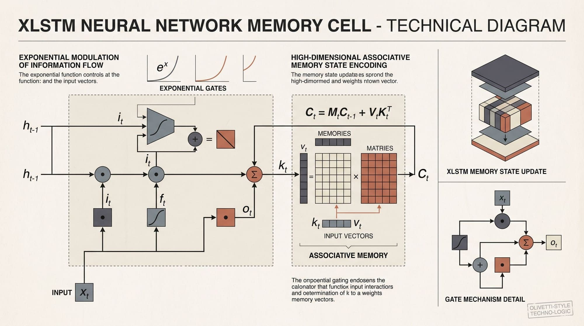
In May 2024, researchers led by Maximilian Beck and Sepp Hochreiter introduced Extended Long Short-Term Memory, or xLSTM (Beck et al., 2024). The architecture addresses the core architectural deficiencies of traditional LSTMs by introducing exponential gating, running normalizer states, and matrix-valued associative memory cells. xLSTM establishes a mathematical duality between recurrent state updates and parallel chunkwise linear attention, enabling parallel training on modern accelerator hardware while retaining constant-memory autoregressive generation.

1. Structural Limitations of Canonical LSTMs

To understand why the canonical LSTM architecture struggled at frontier scale, consider the standard update equations for an LSTM cell at time step $t$:

$$\tilde{z}_t = \tanh(W_z x_t + R_z h_{t-1} + b_z)$$

$$i_t = \sigma(W_i x_t + R_i h_{t-1} + b_i)$$

$$f_t = \sigma(W_f x_t + R_f h_{t-1} + b_f)$$

$$o_t = \sigma(W_o x_t + R_o h_{t-1} + b_o)$$

$$c_t = f_t \odot c_{t-1} + i_t \odot \tilde{z}_t$$

$$h_t = o_t \odot \tanh(c_t)$$

where $x_t \in \mathbb{R}^d$ is the input vector, $c_t \in \mathbb{R}^d$ is the cell state, $h_t \in \mathbb{R}^d$ is the hidden output state, and $\sigma(\cdot)$ denotes the sigmoid activation function.

Three structural limitations restrict this formulation:

1. Inability to Revise Stored Values: The input and forget gates use the sigmoid function $\sigma(z) = \frac{1}{1 + e^{-z}}$, restricting values strictly to $(0, 1)$. When the network processes a critical token early in a context and writes it to cell state $c_t$, subsequent tokens can only scale down the existing memory via $f_t < 1$ or additively superimpose new information via $i_t \odot \tilde{z}_t$. If the model encounters a token that directly contradicts or supersedes past context, it cannot amplify the new incoming value relative to historical state or dynamically reset past state without step-by-step decay.
2. Scalar Memory Capacity Bottleneck: The cell state $c_t$ is a 1D scalar vector of dimension $d$. Information storage scales linearly $O(d)$ with hidden state width. In contrast, multi-head self-attention retains the complete historical Key-Value cache of shape $T \times d$, permitting associative retrieval across all past tokens. A 1D vector cannot bind complex multi-entity relationships without destructive interference across overlapping feature channels.
3. Sequential Training Dependency: The recurrence $h_t = o_t \odot \tanh(c_t)$ feeds directly into the affine transformations of the subsequent step ($R_z h_{t-1}$, $R_i h_{t-1}$, $R_f h_{t-1}$). This hidden-to-hidden recurrence creates an unbroken dependency chain across sequence length $T$. Training cannot be parallelized via matrix multiplications over the time dimension, forcing backpropagation through time (BPTT) and underutilizing GPU tensor cores.

2. sLSTM: Scalar Memory with Exponential Gating and Normalization

The first core building block of xLSTM is the scalar LSTM (sLSTM). The sLSTM preserves a 1D vector cell state but fundamentally alters the gating mechanism and output normalization.

Exponential Gating

Rather than using sigmoid activations, sLSTM equips input and forget gates with exponential functions:

$$i_t = \exp(\tilde{i}_t), \quad \text{where } \tilde{i}_t = W_i x_t + R_i h_{t-1} + b_i$$

$$f_t = \exp(\tilde{f}_t) \quad \text{or} \quad \sigma(\tilde{f}_t)$$

By taking the exponential of the gate pre-activations, the input gate can output values significantly greater than 1. This property allows sLSTM to implement dynamic memory revision: when an incoming token is assigned high relevance, its exponentiated gate weight $i_t$ dominates the accumulated historical state, effectively overriding prior stored values.

The Normalizer State and Numerical Stabilization

Unbounded exponential functions introduce immediate numerical instability and gradient explosions during backpropagation. To stabilize activations, sLSTM introduces a scalar normalizer state $n_t \in \mathbb{R}^d$ and a running maximum tracker $m_t \in \mathbb{R}^d$.

The normalizer state accumulates the history of input gate activations weighted by all subsequent forget gates:

$$n_t = f_t \odot n_{t-1} + i_t$$

The unnormalized cell state is computed as:

$$c_t = f_t \odot c_{t-1} + i_t \odot z_t$$

where $z_t = W_z x_t + R_z h_{t-1} + b_z$ (without the $\tanh$ squashing). The hidden state is then normalized by dividing the cell state by the normalizer state:

$$\tilde{h}_t = \frac{c_t}{n_t}, \quad h_t = o_t \odot \tilde{h}_t$$

To maintain floating-point stability across thousands of steps, sLSTM computes activations in log-space relative to running maximum state $m_t$:

$$m_t = \max(\tilde{f}_t + m_{t-1}, \tilde{i}_t)$$

The stabilized updates then become:

$$c_t = \exp(\tilde{f}_t + m_{t-1} - m_t) \odot c_{t-1} + \exp(\tilde{i}_t - m_t) \odot z_t$$

$$n_t = \exp(\tilde{f}_t + m_{t-1} - m_t) \odot n_{t-1} + \exp(\tilde{i}_t - m_t)$$

This normalization closely mirrors the online softmax trick used in FlashAttention (Dao et al., 2022). It ensures that the elements of $c_t$ and $n_t$ remain numerically bounded while allowing the relative weighting between past context and current input to span multiple orders of magnitude.

Multi-Head Memory Mixing

Unlike traditional LSTMs where hidden dimensions operate independently across cells, sLSTM structures hidden states into multiple heads. Within each head, recurrence is scalar, but across heads, affine projections $R_i, R_f, R_z, R_o$ mix representations. This head-wise communication allows sLSTM to route features dynamically across parallel memory tracks.

3. mLSTM: Matrix Memory and the Parallel Dual Formulation

While sLSTM solves memory revision, its storage capacity remains bounded by $O(d)$. To achieve associative memory storage capable of competing with self-attention, xLSTM introduces the Matrix LSTM (mLSTM).

Associative Matrix Cell State

The mLSTM replaces the scalar cell state $c_t \in \mathbb{R}^d$ with a matrix-valued cell state $C_t \in \mathbb{R}^{d \times d}$.

Input tokens are projected into Query ($q_t$), Key ($k_t$), and Value ($v_t$) vectors:

$$q_t = W_q x_t + b_q$$

$$k_t = \frac{1}{\sqrt{d}} (W_k x_t + b_k)$$

$$v_t = W_v x_t + b_v$$

The matrix memory update utilizes an outer product (covariance update rule) to store Key-Value associations:

$$C_t = f_t C_{t-1} + i_t (v_t k_t^T)$$

where $f_t = \exp(\tilde{f}_t)$ (or $\sigma(\tilde{f}_t)$) and $i_t = \exp(\tilde{i}_t)$. The normalizer state vector $n_t \in \mathbb{R}^d$ accumulates the historical key vectors:

$$n_t = f_t n_{t-1} + i_t k_t$$

Memory retrieval is executed by multiplying the matrix state $C_t$ by the query vector $q_t$:

$$\tilde{h}_t = \frac{C_t q_t}{\max(n_t^T q_t, 1)}$$

$$h_t = o_t \odot \tilde{h}_t$$

By storing information as an outer product $v_t k_t^T$, mLSTM implements a continuous associative memory. Storing multiple key-value pairs in a single matrix $C_t$ enables the network to retrieve specific facts when queried with matching keys, expanding the effective memory capacity from $O(d)$ to $O(d^2)$ per head.

The Parallel Dual Form

In mLSTM, the hidden-to-hidden recurrent connections ($h_{t-1} \to h_t$) are eliminated. Gates and projections depend exclusively on current input $x_t$. This architectural decision unlocks the parallel dual formulation.

Unrolling the matrix recurrence from $t=1$ to $T$:

$$C_T = \sum_{t=1}^T \left( \prod_{\tau=t+1}^T f_\tau \right) i_t v_t k_t^T$$

Evaluating the retrieval at step $T$ with query $q_T$:

$$C_T q_T = \sum_{t=1}^T \left( \prod_{\tau=t+1}^T f_\tau \right) i_t v_t (k_t^T q_T) = \sum_{t=1}^T \left( \prod_{\tau=t+1}^T f_\tau \right) i_t (q_T^T k_t) v_t$$

Let $S \in \mathbb{R}^{T \times T}$ be a causal decay matrix defined by:

$$S_{i,j} = \begin{cases} \left( \prod_{\tau=j+1}^i f_\tau \right) i_j & \text{if } i \ge j \\ 0 & \text{if } i < j \end{cases}$$

The sequence-wide hidden state representation $H \in \mathbb{R}^{T \times d}$ can then be computed entirely in parallel as:

$$H = ( (Q K^T) \odot S ) V$$

This formulation is mathematically equivalent to causal linear attention with exponential decay (Katharopoulos et al., 2020). During training, the entire sequence computation can be executed on tensor cores using parallel associative prefix scans and block-chunked matrix multiplications, identical to chunked algorithms in State Space Models such as Mamba (Gu and Dao, 2023).

4. xLSTM Block Architecture and Residual Stacking

The individual sLSTM and mLSTM cells are integrated into residual blocks to form full deep network architectures.

sLSTM Block Structure

An sLSTM block incorporates convolutional pre-processing and post-up-projection:

1. Layer Normalization: Input $x \in \mathbb{R}^d$ is normalized via LayerNorm or RMSNorm.
2. Causal 1D Convolution: A depthwise causal 1D convolution with small kernel size (e.g., $k=4$) mixes local context across neighboring tokens.
3. sLSTM Cell: The multi-head sLSTM processes the temporally convolved representations.
4. Gated Feed-Forward Projection: The cell output is passed through a GeLU/Swish activation, projected upward to an expanded dimension (e.g., factor 2 or 4), and gated before being projected back to hidden width $d$.
5. Residual Connection: The processed output is added to the skip input.

mLSTM Block Structure

The mLSTM block mirrors modern Transformer decoder and State Space Model blocks:

1. Pre-LayerNorm: Normalizes input $x$.
2. Up-Projection: Projections expand the representation width by expansion factor $p$ (typically $p=2$).
3. Causal 1D Convolution: A depthwise causal 1D convolution acts on Key and Value paths.
4. mLSTM Cell: The matrix memory processes queries, keys, and values across multiple heads.
5. Group Normalization and Output Gating: Output heads are normalized and modulated by output gate $o_t$.
6. Down-Projection and Skip Addition: Projected back to model dimension $d$ and combined with the residual path.

       Input x
          │
    ┌─────┴─────────────────────────┐
    │                               │
[Pre-LN]                         [Skip]
    │                               │
[Up-Projection (2x)]                │
    │                               │
[Causal 1D Conv (k=4)]              │
    │                               │
[mLSTM Matrix Memory Cell]          │
  C_t = f_t C_t-1 + i_t (v_t k_t^T) │
  h_t = (C_t q_t) / (n_t^T q_t)     │
    │                               │
[GroupNorm & Output Gate]           │
    │                               │
[Down-Projection (1/2x)]            │
    │                               │
    ▼                               │
  [ + ] <───────────────────────────┘
    │
 Output y

Hybrid Stacking: xLSTM[a:b] Topologies

Empirical evaluations in Beck et al. (2024) demonstrate that pure mLSTM networks excel at associative memory and global context aggregation, while sLSTM layers excel at tracking state transitions, counting, and non-linear tracking over time.

To combine both capabilities, xLSTM models are constructed as hybrid stacks denoted by xLSTM[a:b], representing the ratio of mLSTM blocks to sLSTM blocks. For instance, an xLSTM[7:1] configuration interleaves seven mLSTM blocks with one sLSTM block throughout the depth of the network.

5. Architectural Comparison: xLSTM vs. Transformers and State Space Models

Comparing xLSTM against dominant foundation model paradigms highlights distinct computational profiles:

• Canonical LSTM: Maintains a 1D state of size $d$. Training is strictly sequential $O(T \cdot d)$, while inference requires $O(1)$ constant time and $O(d)$ memory. Gating is restricted to sigmoid decay with no dynamic revision or outer-product storage.
• Standard Transformer: Retains a full Key-Value cache of shape $T \times d$. Training is fully parallel $O(T^2 \cdot d)$ with exact softmax self-attention. Inference step compute scales with context length $O(T)$, and KV memory grows linearly $O(T \cdot d)$.
• State Space Models (Mamba): Uses a continuous state dimension expanded by factor $N$ (state size $N \cdot d$). Training is parallelized via associative scans in $O(T \cdot d)$ time. Inference requires $O(1)$ constant compute and $O(N \cdot d)$ constant memory per layer.
• xLSTM (mLSTM / sLSTM): Uses an outer-product matrix state of size $d \times d$ (or $H \times d_k \times d_k$) in mLSTM and a 1D vector state in sLSTM. Training is parallelized via chunkwise linear attention scans in $O(T \cdot d)$ time. Inference operates in strictly $O(1)$ constant time and $O(d^2)$ constant memory per layer.

Inference Memory and Throughput Trade-Offs

During autoregressive generation, standard Transformers require maintaining an active KV cache that expands linearly with sequence length $T$ and batch size $B$. For context lengths spanning 32k to 128k tokens, the KV cache dominates GPU High Bandwidth Memory (HBM), necessitating complex paging mechanisms, KV cache compression, and multi-node sharding.

In contrast, xLSTM maintains a constant inference state per layer:

• For sLSTM layers, the state comprises $c_t, n_t, m_t \in \mathbb{R}^d$, requiring $O(d)$ storage.
• For mLSTM layers with $H$ heads each of dimension $d_k$, the state comprises matrix $C_t \in \mathbb{R}^{H \times d_k \times d_k}$ and vector $n_t \in \mathbb{R}^{H \times d_k}$.

Because $C_t$ does not grow with context length $T$, xLSTM executes token generation in strictly $O(1)$ memory and $O(1)$ compute per step. A model processing a 100,000-token prompt occupies the exact same memory footprint during token 100,001 as it did during token 10.

6. Empirical Scaling and Benchmark Results

In the initial 300B-token pre-training evaluations conducted by Beck et al. (2024) across parameter scales from 125M to 1.3B, xLSTM demonstrated competitive performance against strong baseline architectures:

1. Language Modeling Perplexity: xLSTM achieved lower validation perplexity on the SlimPajama corpus compared to open-source Transformer architectures (including LLaMA configurations) and State Space Models (Mamba and RWKV-4/5) at matched compute budgets.
2. Associative Recall Tasks: In synthetic multi-query associative recall (MQAR) benchmarks, canonical LSTMs fail completely once sequence length exceeds a few hundred tokens. mLSTM maintained 100% retrieval accuracy across long sequence contexts, matching full softmax attention up to the tested limits.
3. Long Context Extrapolation: Due to exponential gating and running normalizer states, xLSTM exhibited stable perplexity curves when evaluated on sequences longer than its training context window, avoiding the catastrophic loss degradation common in un-windowed recurrent networks.

Subsequent work scaling the architecture to 7 billion parameters (Beck et al., 2025) confirmed that these scaling properties hold at production scale, demonstrating high throughput on GPU clusters when training with chunkwise kernel implementations.

7. Summary of Core Principles

The xLSTM architecture revitalizes recurrent neural networks for foundation model workloads through four primary innovations:

• Exponential Gating: Replaces bounded sigmoid gates with exponential functions, granting the network the mathematical expressivity to revise stored memory dynamically.
• Normalizer and Max States: Introduces running denominator $n_t$ and maximum tracker $m_t$ to prevent numerical overflow, stabilizing training across deep stacks.
• Associative Matrix Memory (mLSTM): Upgrades scalar storage to outer-product key-value matrix accumulation ($C_t = f_t C_{t-1} + i_t v_t k_t^T$), expanding memory capacity to $O(d^2)$.
• Parallel Dual Formulation: Drops recurrent hidden-to-hidden connections in mLSTM, enabling $O(T)$ chunked parallel training via associative scans while preserving $O(1)$ constant-memory autoregressive inference.

Sources

• Beck, M., Pöppel, K., Spanring, M., Auer, A., Prudnikova, O., Kopp, M. K., Klambauer, G., Brandstetter, J., and Hochreiter, S. (2024). xLSTM: Extended Long Short-Term Memory. arXiv:2405.04517.
• Beck, M., Pöppel, K., Lippe, P., Kurle, R., Blies, P. M., Klambauer, G., Böck, S., and Hochreiter, S. (2025). xLSTM 7B: A Recurrent LLM for Fast and Efficient Inference. arXiv:2503.13427.
• Hochreiter, S., and Schmidhuber, J. (1997). Long Short-Term Memory. Neural Computation, 9(8), 1735-1780. Bioinf JKU Publication Archive.
• Vaswani, A., Shazeer, N., Parmar, N., Uszkoreit, J., Jones, L., Gomez, A. N., Kaiser, Ł., and Polosukhin, I. (2017). Attention Is All You Need. arXiv:1706.03762.
• Dao, T., Fu, D. Y., Ermon, S., Rudra, A., and Ré, C. (2022). FlashAttention: Fast and Memory-Efficient Exact Attention with IO-Awareness. arXiv:2205.14135.
• Gu, A., and Dao, T. (2023). Mamba: Linear-Time Sequence Modeling with Selective State Spaces. arXiv:2312.00752.
• Katharopoulos, A., Vyas, A., Pappas, N., and Fleuret, F. (2020). Transformers are RNNs: Fast Autoregressive Transformers with Linear Attention. arXiv:2006.16236.