Transformer Feed-Forward Networks as Key-Value Memories: How First-Layer Keys and Second-Layer Values Store Knowledge

In modern autoregressive Transformers, the division of labor between attention heads and multi-layer perceptron (MLP) blocks is often summarized through a clean functional split: attention routes information across sequence positions, while feed-forward networks (FFNs) process information per position. Yet for years, the exact mechanism by which FFNs process that information remained a black box.

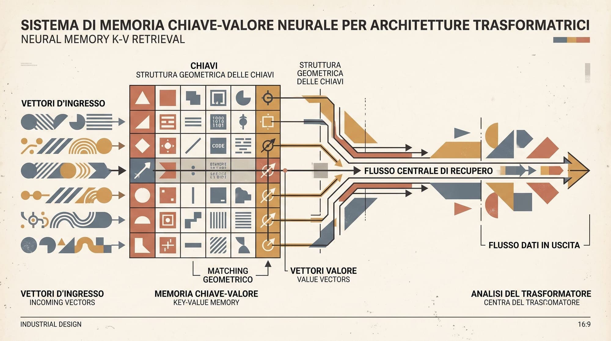
Foundational interpretability research by Geva et al. (2021) demonstrated that Transformer feed-forward networks operate mathematically as unnormalized associative key-value memories. Under this formulation:

1. The first linear layer acts as a bank of pattern-matching keys ($W_1$) that detect textual, syntactic, or semantic triggers in the input representation.
2. The non-linear activation function serves as a thresholding and routing filter.
3. The second linear layer acts as a bank of values ($W_2$) whose corresponding vectors are retrieved, weighted, and written directly into the model's residual stream.

Understanding this key-value memory formulation explains why FFNs account for roughly two-thirds of a Transformer's total non-embedding parameter budget, how factual knowledge is localized across layers, and how techniques like model editing and Mixture of Experts scale LLM capacity.

The Mathematical Isomorphism: FFN as Associative Lookup

In a standard Transformer block, the feed-forward sublayer processes an incoming hidden vector $x \in \mathbb{R}^{d_{\text{model}}}$ from the residual stream. The standard two-layer MLP computation is defined as:

$$\text{FFN}(x) = \sigma(x W_1 + b_1) W_2 + b_2$$

where $W_1 \in \mathbb{R}^{d_{\text{model}} \times d_{\text{ff}}}$, $W_2 \in \mathbb{R}^{d_{\text{ff}} \times d_{\text{model}}}$, $b_1 \in \mathbb{R}^{d_{\text{ff}}}$, $b_2 \in \mathbb{R}^{d_{\text{model}}}$, and $\sigma(\cdot)$ is a non-linear activation function (such as GELU or ReLU). The intermediate dimension $d_{\text{ff}}$ is typically set to $4 d_{\text{model}}$ in standard architectures (or $\frac{8}{3} d_{\text{model}}$ in gated variants such as SwiGLU).

To see the key-value memory structure, let:

• $k_i \in \mathbb{R}^{d_{\text{model}}}$ denote the $i$-th column of $W_1$ (the $i$-th key vector, for $i \in \{1, \dots, d_{\text{ff}}\}$).
• $v_i \in \mathbb{R}^{d_{\text{model}}}$ denote the $i$-th row of $W_2$ (the $i$-th value vector).
• $b_{1,i} \in \mathbb{R}$ denote the $i$-th scalar bias in $b_1$.

Expanding the matrix multiplication into vector operations yields:

$$\text{FFN}(x) = \sum_{i=1}^{d_{\text{ff}}} \sigma(x \cdot k_i + b_{1,i}) v_i + b_2$$

This formulation matches the mathematical definition of an associative key-value memory:

1. Key Matching (Addressing): The inner product $x \cdot k_i$ measures the similarity between the current hidden state $x$ and the $i$-th key vector $k_i$.
2. Activation Filtering: The scalar activation $m_i(x) = \sigma(x \cdot k_i + b_{1,i})$ determines how strongly memory slot $i$ fires.
3. Value Retrieval and Superposition: The output is a linear combination of value vectors $\sum_i m_i(x) v_i$, where each value vector $v_i$ is injected in proportion to its activation intensity.

Unlike attention-based key-value retrieval, which normalizes coefficients via softmax across tokens in a context window, the FFN memory operates independently per token across $d_{\text{ff}}$ discrete memory slots using elementwise activations.

Keys as Pattern Detectors, Values as Vocabulary Concepts

What do individual keys and values actually represent? Subsequent mechanistic work by Geva et al. (2022) and Dai et al. (2022) systematically analyzed the inputs that activate specific neurons and the output distributions induced by their corresponding value vectors.

Keys as Trigger Patterns

By tracking which text prefixes produce the largest inner product $x \cdot k_i$, researchers found that individual keys act as specialized pattern detectors:

• Shallow Patterns: Keys in early layers trigger on specific n-grams, capitalization, punctuation formats, or morphological suffixes (such as words ending in "-ing" or capitalized acronyms).
• Semantic Classes: Keys in middle layers trigger on conceptual categories, such as mentions of programming languages, geographical locations, or corporate entities.
• Relational Contexts: Keys in upper-middle layers trigger on specific relational prompts (such as "The capital of [Country] is" or "authored by").

Values as Vocabulary Directions

Because each value vector $v_i \in \mathbb{R}^{d_{\text{model}}}$ lives in the same hidden space as the residual stream, it can be directly analyzed by projecting it through the language model's unembedding matrix $W_U \in \mathbb{R}^{d_{\text{model}} \times |V|}$ (often termed the Logit Lens):

$$\text{logits}(v_i) = v_i W_U$$

When projected into vocabulary space, individual value vectors $v_i$ place high probability mass on a small, semantically coherent cluster of tokens. For instance:

• A key $k_i$ that activates on phrases describing the Eiffel Tower or the Louvre pairs with a value vector $v_i$ that directly boosts the logits for "Paris", "France", and "French".
• A key $k_i$ that detects code definitions pairs with a value vector $v_i$ that promotes programming syntax tokens such as return, def, or import.

Feed-forward layers function by querying these memory slots and adding their output directly to the residual stream:

$$x_{l+1} = x_l + \text{Attn}(x_l) + \sum_{i=1}^{d_{\text{ff}}} m_i(x_l) v_i$$

Each layer sequentially modifies the token distribution by promoting or suppressing specific vocabulary candidates.

Layerwise Specialization: The Three-Tier Memory Hierarchy

Across a multi-layer Transformer, the functional role of key-value memories evolves systematically from lower to upper layers:

| Layer Tier | Representation Level | Key Triggers ($k_i$) | Value Vector Output ($v_i W_U$) | | :--- | :--- | :--- | :--- | | Lower Layers (0 to 30%) | Surface & Syntax | Token prefixes, casing, syntax markers, subword concatenations | Syntactic continuations, morphological completions | | Middle Layers (30 to 70%) | Semantics & Knowledge | Entity types, subject-relation tuples, relational contexts | Factual attributes, related entity names, topical terms | | Upper Layers (70 to 100%) | Prediction & Distribution | Task-specific goals, next-token formatting context | Exact next-token candidates, probability mass sharpening |

In research exploring knowledge localization, Meng et al. (2022) demonstrated via causal tracing that factual recall (such as determining the country associated with a landmark) originates in the early-to-middle MLP layers at the subject token position, which is then routed to the final sequence position by late attention layers.

The Parameter Budget and SwiGLU Gating

Feed-forward layers represent the largest parameter footprint in standard language models. In a vanilla Transformer with hidden dimension $d_{\text{model}}$ and $d_{\text{ff}} = 4 d_{\text{model}}$:

• Self-Attention Sublayer: $W_Q, W_K, W_V, W_O \in \mathbb{R}^{d_{\text{model}} \times d_{\text{model}}}$ account for $4 d_{\text{model}}^2$ parameters.
• FFN Sublayer: $W_1 \in \mathbb{R}^{d_{\text{model}} \times 4 d_{\text{model}}}$ and $W_2 \in \mathbb{R}^{4 d_{\text{model}} \times d_{\text{model}}}$ account for $8 d_{\text{model}}^2$ parameters.

Thus, FFN blocks consume $\frac{8}{12} = 66.7\%$ of total transformer layer weights (excluding embeddings).

Standard FFN (2-Layer MLP):
Input x ────────────────────────┬───────────────────────────┐
                                │                           │
                                ▼                           │
                        [ Key Matrix W₁ ]                   │
                                │ (x · k_i)                 │
                                ▼                           │
                        [ Activation σ ]                    │
                                │ (m_i)                     │
                                ▼                           │
                       [ Value Matrix W₂ ]                  │
                                │ (Σ m_i · v_i)             │
                                ▼                           │
                               ( + ) ◄──────────────────────┘ (Residual Stream)
                                │
                              Output

SwiGLU Gating Architecture

Modern architectures (such as LLaMA, Mistral, and Qwen) replace the two-matrix MLP with SwiGLU (Shazeer, 2020), which introduces an explicit multiplicative gating branch:

$$\text{SwiGLU}(x) = \left( \text{Swish}(x W_{\text{gate}}) \odot x W_{\text{up}} \right) W_{\text{down}}$$

To maintain a comparable parameter budget of $8 d_{\text{model}}^2$, $d_{\text{ff}}$ is scaled down to approximately $\frac{8}{3} d_{\text{model}}$:

$$\text{Parameters} = 3 \times d_{\text{model}} \times \left(\frac{8}{3} d_{\text{model}}\right) = 8 d_{\text{model}}^2$$

Under the key-value interpretation, the gating branch $\text{Swish}(x W_{\text{gate}})$ provides a dynamic continuous gate that scales the projection $x W_{\text{up}}$ before the linear value recombination in $W_{\text{down}}$, increasing memory capacity per parameter without increasing inference FLOPs.

Practical Applications: Model Editing and Mixture of Experts

Viewing FFN layers as associative memories is not merely an interpretability framework; it has enabled practical architectural and operational capabilities:

1. Rank-One Model Editing (ROME) and MEMIT

Because the second linear layer $W_2$ serves as a linear value lookup matrix satisfying $W_2 K \approx V$, researchers can treat factual editing as a constrained linear algebra problem. Meng et al. (2022) and Meng et al. (2023) demonstrated that injecting a new fact (or updating an existing one) can be executed in closed form using a rank-one weight update:

$$\Delta W_2 = (v^* - W_2 k^<em>) (C^{-1} k^</em>)^T$$

where $k^$ is the key vector for the target subject entity, $v^$ is the desired value vector corresponding to the target property, and $C$ is a covariance matrix of unperturbed key activations that prevents catastrophic forgetting.

2. Mixture of Experts (MoE)

The key-value memory perspective explains why Mixture of Experts architectures (such as Mixtral, DeepSeek-V3, and Grok) scale model capacity by replicating FFN layers while keeping attention layers shared:

• FFN parameters store static knowledge and associative facts.
• Attention parameters govern dynamic contextual routing.

By partitioning the FFN key-value memory banks into discrete routed experts ($E_1, \dots, E_N$), models can expand total factual memory capacity to hundreds of billions of parameters while only activating top-$k$ memory banks per token, keeping active inference latency and FLOPs constant.

Sources

• Geva et al. (2021): Transformer Feed-Forward Layers Are Key-Value Memories
• Geva et al. (2022): Transformer Feed-Forward Layers Build Predictions by Promoting Concepts in the Vocabulary
• Dai et al. (2022): Knowledge Neurons in Pretrained Transformers
• Meng et al. (2022): Locating and Editing Factual Associations in GPT (ROME)
• Meng et al. (2023): Mass-Editing Memory in a Transformer (MEMIT)
• Shazeer (2020): GLU Variants Improve Transformer