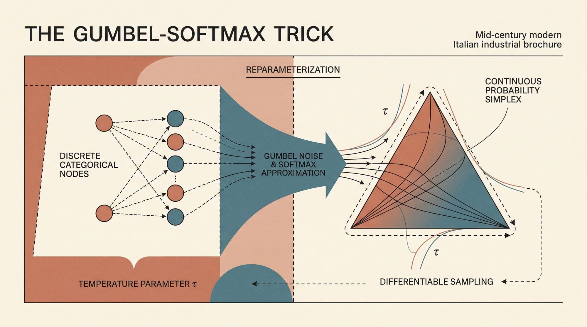
The Gumbel-Softmax Trick: How Continuous Relaxations Enable Differentiable Discrete Sampling

In modern deep learning, end-to-end training depends on reverse-mode automatic differentiation. When an architecture operates on continuous tensors, computing gradients via the chain rule is straightforward. However, many foundational artificial intelligence problems involve discrete choices: selecting tokens from a fixed vocabulary, routing tokens to expert networks in a Mixture-of-Experts (MoE) architecture, activating discrete graph edges, or learning symbolic latent representations.

Standard discrete sampling operations introduce non-differentiable bottlenecks. Evaluating a discrete sample via an argmax or multinomial draw yields zero gradients almost everywhere and undefined gradients at decision boundaries. To optimize parameters upstream of discrete operations, practitioners historically relied on high-variance score-function estimators such as REINFORCE.

The Gumbel-Softmax distribution (simultaneously introduced as the Concrete distribution by Jang, Gu, and Poole, 2016 and Maddison, Mnih, and Teh, 2016) resolved this challenge. By combining the classical Gumbel-Max reparameterization trick with a temperature-controlled continuous relaxation, Gumbel-Softmax provides low-variance, pathwise gradient estimates through discrete categorical distributions.

The Discrete Sampling Bottleneck

Consider a parameterized categorical distribution over $K$ discrete classes with unnormalized log-probabilities (logits) $\boldsymbol{\alpha} = (\alpha_1, \alpha_2, \dots, \alpha_K) \in \mathbb{R}^K$. The class probabilities $\boldsymbol{\pi} = (\pi_1, \dots, \pi_K)$ are given by the standard softmax function:

$$\pi_i = \frac{\exp(\alpha_i)}{\sum_{j=1}^K \exp(\alpha_j)}$$

Let $z$ be a discrete random variable sampled from this categorical distribution:

$$z \sim \text{Categorical}(\boldsymbol{\pi})$$

When $z$ is parameterized as a one-hot indicator vector $\boldsymbol{d} \in \{0, 1\}^K$ where $d_i = 1$ if $z = i$ and $d_i = 0$ otherwise, the expected loss under a downstream objective function $f(\boldsymbol{d})$ parameterized by $\boldsymbol{\theta}$ is:

$$\mathcal{L}(\boldsymbol{\alpha}) = \mathbb{E}_{\boldsymbol{d} \sim p_{\boldsymbol{\alpha}}(\boldsymbol{d})}[f(\boldsymbol{d})]$$

To minimize this loss with gradient-based optimizers, we require the gradient with respect to the input logits $\nabla_{\boldsymbol{\alpha}} \mathcal{L}(\boldsymbol{\alpha})$. Because the discrete sampling step $\boldsymbol{d} \sim \text{Categorical}(\boldsymbol{\pi})$ is a step function, standard backpropagation fails:

$$\frac{\partial \boldsymbol{d}}{\partial \alpha_i} = \mathbf{0} \quad \text{almost everywhere}$$

The Limitations of Score-Function Estimators

Before continuous relaxations, the standard approach to optimize discrete expectations was the score-function estimator (also known as the Likelihood Ratio method or REINFORCE; Williams, 1992):

$$\nabla_{\boldsymbol{\alpha}} \mathbb{E}_{\boldsymbol{d} \sim p_{\boldsymbol{\alpha}}(\boldsymbol{d})}[f(\boldsymbol{d})] = \mathbb{E}_{\boldsymbol{d} \sim p_{\boldsymbol{\alpha}}(\boldsymbol{d})}[f(\boldsymbol{d}) \nabla_{\boldsymbol{\alpha}} \log p_{\boldsymbol{\alpha}}(\boldsymbol{d})]$$

While REINFORCE provides an unbiased gradient estimator, it suffers from severe variance. The term $f(\boldsymbol{d})$ scales the score function directly; if the downstream reward or loss fluctuates, gradient estimates exhibit enormous noise. Complex control variates, baseline subtractions, and variance reduction methods (such as NVIL, MuProp, and REBAR; Tucker et al., 2017) reduce this variance, but at the cost of additional model components, auxiliary training runs, and high implementation complexity.

The Gumbel-Max Reparameterization

To understand Gumbel-Softmax, we first examine the Gumbel-Max trick (Gumbel, 1954; Luce, 1959; McFadden, 1974), which provides a method to draw discrete categorical samples via deterministic transformations of continuous noise.

The Standard Gumbel distribution $\text{Gumbel}(0, 1)$ has the cumulative distribution function (CDF) and probability density function (PDF):

$$F(g) = \exp(-\exp(-g))$$

$$f(g) = \exp(-(g + \exp(-g)))$$

To draw independent and identically distributed (i.i.d.) samples from $\text{Gumbel}(0, 1)$, we apply inverse transform sampling to uniform random variables $u \sim \text{Uniform}(0, 1)$:

$$g = -\log(-\log(u))$$

Mathematical Proof of the Gumbel-Max Trick

Let $\boldsymbol{\alpha} = (\alpha_1, \dots, \alpha_K)$ be logits corresponding to probabilities $\pi_i = \frac{\exp(\alpha_i)}{\sum_j \exp(\alpha_j)}$, and let $g_1, \dots, g_K \sim \text{Gumbel}(0, 1)$ be independent Gumbel perturbations. Define the discrete index $z$:

$$z = \arg\max_{i \in \{1, \dots, K\}} (\alpha_i + g_i)$$

To prove that $P(z = k) = \pi_k$, consider the condition where $\alpha_k + g_k$ exceeds all other perturbed logits $\alpha_i + g_i$ for $i \neq k$:

$$P(z = k) = P\left(\bigcap_{i \neq k} (\alpha_i + g_i < \alpha_k + g_k)\right)$$

Conditioning on a fixed value of $g_k = g$:

$$P(z = k \mid g_k = g) = \prod_{i \neq k} P(g_i < g + \alpha_k - \alpha_i) = \prod_{i \neq k} \exp\left(-\exp(-(g + \alpha_k - \alpha_i))\right)$$

Combining terms inside the exponent:

$$P(z = k \mid g_k = g) = \exp\left(-\sum_{i \neq k} \exp(-(g + \alpha_k - \alpha_i))\right) = \exp\left(-\exp(-g) \sum_{i \neq k} \exp(\alpha_i - \alpha_k)\right)$$

Integrating over the density $f(g) = \exp(-g - \exp(-g))$ of $g_k$:

$$P(z = k) = \int_{-\infty}^{\infty} \exp\left(-\exp(-g) \sum_{i \neq k} \exp(\alpha_i - \alpha_k)\right) \exp(-g - \exp(-g)) \, dg$$

Factoring out $\exp(-g)$:

$$P(z = k) = \int_{-\infty}^{\infty} \exp(-g) \exp\left(-\exp(-g) \left[ 1 + \sum_{i \neq k} \exp(\alpha_i - \alpha_k) \right]\right) dg$$

Recognizing that $1 + \sum_{i \neq k} \exp(\alpha_i - \alpha_k) = \sum_{i=1}^K \exp(\alpha_i - \alpha_k) = \frac{\sum_{i=1}^K \exp(\alpha_i)}{\exp(\alpha_k)}$:

$$P(z = k) = \int_{-\infty}^{\infty} \exp(-g) \exp\left(-\exp(-g) \frac{\sum_{i=1}^K \exp(\alpha_i)}{\exp(\alpha_k)}\right) dg$$

Using the substitution $v = \exp(-g)$ (where $dv = -\exp(-g)dg$):

$$P(z = k) = \int_{0}^{\infty} \exp\left(-v \frac{\sum_{i=1}^K \exp(\alpha_i)}{\exp(\alpha_k)}\right) dv = \frac{\exp(\alpha_k)}{\sum_{i=1}^K \exp(\alpha_i)} = \pi_k$$

The Gumbel-Max trick separates the source of stochasticity (the noise vector $\boldsymbol{g}$) from the distribution parameters $\boldsymbol{\alpha}$. However, because the $\arg\max$ operation remains non-differentiable, we cannot compute pathwise derivatives through it.

Continuous Relaxation: The Gumbel-Softmax Distribution

The core insight of the Gumbel-Softmax (Concrete) distribution is to replace the non-differentiable $\arg\max$ operator with a continuous, temperature-parameterized $\text{softmax}$ function.

Instead of outputting a discrete index $z \in \{1, \dots, K\}$, we generate a continuous random vector $\boldsymbol{y} = (y_1, y_2, \dots, y_K)$ lying on the open $(K-1)$-dimensional probability simplex:

$$\Delta^{K-1} = \left\{ \boldsymbol{y} \in \mathbb{R}^K \;\middle|\; \sum_{i=1}^K y_i = 1, \; y_i > 0 \right\}$$

Each coordinate $y_i$ is computed as:

$$y_i = \frac{\exp\left(\frac{\alpha_i + g_i}{\tau}\right)}{\sum_{j=1}^K \exp\left(\frac{\alpha_j + g_j}{\tau}\right)}$$

where:

• $\alpha_i = \log \pi_i$ is the unnormalized logit for class $i$.
• $g_i = -\log(-\log(u_i))$ with $u_i \sim \text{Uniform}(0, 1)$ are i.i.d. Standard Gumbel noise samples.
• $\tau \in (0, \infty)$ is the temperature hyperparameter.

+---------------------+     +--------------------+
| Unnormalized Logits |     | Standard Gumbel    |
|       alpha_i       |     | Noise  g_i ~ G(0,1)|
+----------+----------+     +---------+----------+
           |                          |
           +------------+-------------+
                        |
                        v
              [ (alpha_i + g_i) / tau ]
                        |
                        v
             +--------------------+
             |  Softmax Operator  |
             +----------+---------+
                        |
                        v
     Continuous Simplex Vector: y in Delta^{K-1}

Simplex Density Function

As derived by Maddison et al., 2016, the probability density function of the Concrete / Gumbel-Softmax distribution over the interior of the simplex $\Delta^{K-1}$ with parameters $\boldsymbol{\alpha} = (\alpha_1, \dots, \alpha_K)$ and temperature $\tau$ is given by:

$$p_{\boldsymbol{\alpha}, \tau}(\boldsymbol{y}) = (K - 1)! \, \tau^{K-1} \left( \sum_{i=1}^K \frac{\exp(\alpha_i)}{y_i^\tau} \right)^{-K} \prod_{i=1}^K \frac{\exp(\alpha_i)}{y_i^{\tau+1}}$$

This density has a closed form, allowing analytical evaluation of log-likelihoods when required in probabilistic models.

Temperature Dynamics and the Bias-Variance Trade-Off

The temperature parameter $\tau$ dictates the geometric behavior of the sample $\boldsymbol{y}$ across the simplex and governs the fundamental trade-off between gradient bias and gradient variance.

       tau -> infinity                      tau = 1.0                      tau -> 0+
  (Uniform Center Point)             (Smooth Continuous Cloud)      (Hard One-Hot Vertices)
  
          (0,1,0)                            (0,1,0)                        (0,1,0)
             ^                                  ^                              ^
            / \                                / \                            / \
           /   \                              / . \                          /   \
          /  *  \                            / ... \                        *     \
         /       \                          / . * . \                      /       \
        +---------+                        +---------+                    +---------*
     (1,0,0)   (0,0,1)                  (1,0,0)   (0,0,1)              (1,0,0)   (0,0,1)
  
  * Low Gradient Variance            * Balanced Regime              * Zero Approximation Bias
  * High Approximation Bias          * Stable Optimization          * Exploding Gradient Variance

1. High-Temperature Limit ($\tau \to \infty$)

As $\tau \to \infty$, the term $\frac{\alpha_i + g_i}{\tau} \to 0$ for all $i$. The exponentiated values converge to 1, causing the output vector to collapse to the simplex centroid:

$$\lim_{\tau \to \infty} y_i = \frac{1}{K}$$

In this regime, the output vector carries little dependence on the underlying logits $\boldsymbol{\alpha}$ or noise $\boldsymbol{g}$. The gradient $\nabla_{\boldsymbol{\alpha}} \boldsymbol{y}$ is smooth and has near-zero variance, but the approximation bias relative to a discrete categorical distribution is maximal.

2. Low-Temperature Limit ($\tau \to 0^+$)

As $\tau \to 0^+$, the softmax behaves as a hard $\arg\max$. The coordinate with the largest perturbed logit $\alpha_k + g_k$ dominates all others exponentially:

$$\lim_{\tau \to 0^+} y_i = \begin{cases} 1 & \text{if } i = \arg\max_j (\alpha_j + g_j) \\ 0 & \text{otherwise} \end{cases}$$

In this limit, the continuous sample converges in distribution to the exact one-hot categorical sample:

$$\lim_{\tau \to 0^+} \boldsymbol{y} \stackrel{d}{=} \boldsymbol{d} \sim \text{Categorical}(\boldsymbol{\pi})$$

Approximation bias is zero, but the derivative $\frac{\partial y_i}{\partial \alpha_j}$ approaches Dirac delta impulses at decision boundaries and zero elsewhere, causing gradient variance to explode.

3. Temperature Annealing Schedules

To balance exploration early in training with discrete fidelity late in training, practitioners apply temperature annealing schedules. Common formulations include:

• Exponential Annealing:

$$\tau_t = \max\left(\tau_{\min}, \; \tau_0 \cdot \exp(-r \cdot t)\right)$$

• Cosine Annealing:

$$\tau_t = \tau_{\min} + \frac{1}{2}(\tau_0 - \tau_{\min})\left(1 + \cos\left(\frac{\pi t}{T}\right)\right)$$

Typical initial values range from $\tau_0 \in [1.0, 2.0]$, cooling down to $\tau_{\min} \in [0.1, 0.5]$ across training iterations $t$.

The Straight-Through (ST) Gumbel-Softmax Estimator

While the standard Gumbel-Softmax distribution yields continuous vectors $\boldsymbol{y} \in \Delta^{K-1}$, many neural network layers require strictly discrete, one-hot inputs. For instance, lookup tables in token embeddings or discrete hardware routing units cannot accept fractional mixtures.

The Straight-Through (ST) Gumbel-Softmax estimator bridges this requirement by decoupling the forward evaluation from the backward gradient calculation:

1. Forward Pass: Compute continuous soft probabilities $\boldsymbol{y}_{\text{soft}}$ using the Gumbel-Softmax formula, then apply a hard discretization:

$$z = \arg\max_{i} (y_{\text{soft}, i}) = \arg\max_i (\alpha_i + g_i)$$ $$\boldsymbol{y}_{\text{hard}} = \text{one\_hot}(z) \in \{0, 1\}^K$$ Feed $\boldsymbol{y}_{\text{hard}}$ into the downstream computation $f(\boldsymbol{y}_{\text{hard}})$.

1. Backward Pass: During backpropagation, bypass the non-differentiable $\arg\max$ and backpropagate gradients directly through the continuous vector $\boldsymbol{y}_{\text{soft}}$:

$$\nabla_{\boldsymbol{\alpha}} f(\boldsymbol{y}_{\text{hard}}) \approx \nabla_{\boldsymbol{\alpha}} \boldsymbol{y}_{\text{soft}} \cdot \left( \nabla_{\boldsymbol{y}_{\text{hard}}} f(\boldsymbol{y}_{\text{hard}}) \right)$$

Computational Implementation Trick

In automatic differentiation frameworks (such as PyTorch or JAX), the Straight-Through estimator is implemented using a stop-gradient operator without manual backward hooks:

$$\boldsymbol{y}_{\text{ST}} = \boldsymbol{y}_{\text{hard}} - \text{stop\_gradient}(\boldsymbol{y}_{\text{soft}}) + \boldsymbol{y}_{\text{soft}}$$

In the forward pass: $$\boldsymbol{y}_{\text{ST}} = \boldsymbol{y}_{\text{hard}} - \boldsymbol{y}_{\text{soft}} + \boldsymbol{y}_{\text{soft}} = \boldsymbol{y}_{\text{hard}}$$

In the backward pass: $$\nabla_{\boldsymbol{\alpha}} \boldsymbol{y}_{\text{ST}} = \mathbf{0} - \mathbf{0} + \nabla_{\boldsymbol{\alpha}} \boldsymbol{y}_{\text{soft}} = \nabla_{\boldsymbol{\alpha}} \boldsymbol{y}_{\text{soft}}$$

Comparison of Gradient Estimators for Discrete Variables

Choosing a gradient estimator for stochastic or discrete computations requires balancing gradient bias, variance, computational cost, and implementation overhead.

| Estimator | Form / Mechanism | Gradient Bias | Gradient Variance | Forward Output | Primary Use Case | | :--- | :--- | :--- | :--- | :--- | :--- | | Score Function (REINFORCE) | $f(z) \nabla_{\boldsymbol{\theta}} \log p(z)$ | Zero (Unbiased) | Very High | Discrete | Black-box rewards, RL environments | | REBAR / RELAX | REINFORCE + Concrete Control Variates | Zero (Unbiased) | Moderate | Discrete | High-precision variational inference | | Gumbel-Softmax (Continuous) | $\nabla_{\boldsymbol{\theta}} f(\boldsymbol{y}_{\text{soft}}(\boldsymbol{\theta}, \boldsymbol{g}))$ | Non-zero (when $\tau > 0$) | Low | Continuous Simplex | Differentiable architecture search, soft routing | | Straight-Through Gumbel-Softmax | Forward $\boldsymbol{y}_{\text{hard}}$, Backward $\boldsymbol{y}_{\text{soft}}$ | Moderate | Low to Moderate | Discrete (One-Hot) | Discrete VAEs, token selection, sparse MoE | | Vector Quantization (VQ-VAE) | Nearest-Neighbor Codebook + Copy Gradients | Heuristic | Low | Discrete Index | Image/audio tokenizers (VQGAN, SoundStream) |

Applications Across Modern AI and LLM Systems

1. Categorical Variational Autoencoders (Discrete VAEs)

Continuous Gaussian latent spaces $\boldsymbol{z} \sim \mathcal{N}(\boldsymbol{\mu}, \boldsymbol{\Sigma})$ can suffer from posterior collapse in autoencoders paired with powerful autoregressive decoders. Discrete latent spaces force models to represent distinct semantic clusters. By placing Gumbel-Softmax distributions over latent codebooks, models learn discrete representations end-to-end without needing complex vector-quantization lookup routines.

2. Sparse Mixture-of-Experts (MoE) Routing and Load Balancing

In large Mixture-of-Experts models (such as Switch Transformer, Mixtral, and DeepSeek-V3), routing networks assign input tokens to top-$k$ expert sub-networks. Deterministic top-$k$ routing can lead to routing collapse, where a small subset of experts receives all tokens while others remain unutilized. Introducing Gumbel noise to routing logits encourages exploration across the expert pool during training:

$$\text{Routing Scores} = \text{TopK}\left(\text{Softmax}\left(\frac{\boldsymbol{W}_r \boldsymbol{x} + \boldsymbol{g}}{\tau}\right), \; k\right)$$

3. Differentiable Discrete Prompt and Token Optimization

Discrete prompt optimization (searching for token sequences that steer language models or trigger specific behaviors) is combinatorially difficult. Rather than evaluating exponential discrete combinations, researchers parameterize prompt tokens as Gumbel-Softmax distributions over the model vocabulary. This enables gradient descent to optimize prompts directly through the token embedding matrix before annealing down to hard vocabulary indices.

4. Differentiable Neural Architecture Search (DARTS)

In automated architecture search, continuous relaxations allow gradient descent to optimize categorical subgraph selections (such as choosing between a $3 \times 3$ convolution, $5 \times 5$ convolution, or identity connection) simultaneously with network weights, reducing search compute from thousands of GPU hours to single-digit runs.

Production Implementation Patterns

When implementing Gumbel-Softmax in production systems, numerical stability is essential. Drawing uniform random numbers near 0 or 1 can produce NaN or -inf values when computing nested logarithms.

Stable PyTorch Implementation

import torch
import torch.nn as nn
import torch.nn.functional as F

def sample_gumbel(shape: torch.Size, eps: float = 1e-20, device: torch.device = None) -> torch.Tensor:
    """
    Sample standard Gumbel noise g ~ Gumbel(0, 1) using inverse transform sampling.
    Clamps uniform samples to prevent log(0) numerical instabilities.
    """
    u = torch.rand(shape, device=device)
    # Clamp to prevent log(0)
    u = torch.clamp(u, min=eps, max=1.0 - eps)
    return -torch.log(-torch.log(u))

def gumbel_softmax_sample(logits: torch.Tensor, temperature: float, eps: float = 1e-20) -> torch.Tensor:
    """
    Add Gumbel noise to logits and apply temperature-scaled softmax.
    """
    g = sample_gumbel(logits.size(), eps=eps, device=logits.device)
    perturbed_logits = (logits + g) / temperature
    return F.softmax(perturbed_logits, dim=-1)

def custom_gumbel_softmax(
    logits: torch.Tensor, 
    temperature: float = 1.0, 
    hard: bool = False, 
    eps: float = 1e-20
) -> torch.Tensor:
    """
    Complete Gumbel-Softmax operator supporting continuous relaxation
    and Straight-Through (hard=True) discretization.
    """
    y_soft = gumbel_softmax_sample(logits, temperature, eps=eps)
    
    if not hard:
        return y_soft
    
    # Straight-Through discretization
    index = y_soft.argmax(dim=-1, keepdim=True)
    y_hard = torch.zeros_like(logits).scatter_(-1, index, 1.0)
    
    # Straight-Through gradient trick: forward is y_hard, backward is y_soft
    return y_hard - y_soft.detach() + y_soft

Key Numerical Guardrails

1. Epsilon Clamping: Always clamp uniform samples $u \in [\epsilon, 1 - \epsilon]$ with $\epsilon \approx 10^{-20}$ before applying $-\log(-\log(u))$. If $u = 0$, $\log(u) = -\infty$, resulting in $\log(\infty) = \text{NaN}$. If $u = 1$, $-\log(u) = 0$, resulting in $\log(0) = -\infty$.
2. Logit Scaling: Maintain input logits $\boldsymbol{\alpha}$ in unnormalized log-space. Applying $\text{Softmax}$ before adding Gumbel noise degrades numerical precision due to catastrophic cancellation in floating-point exponents.
3. Minimum Temperature Floor: When annealing temperature $\tau$, enforce a lower bound $\tau_{\min} \ge 0.1$. Below $0.1$, floating-point division by $\tau$ can overflow standard FP16 and BF16 numerical ranges ($> 65504$ in FP16), leading to infinite logits and gradient underflow.

Sources

• Jang, E., Gu, S., & Poole, B. (2016). Categorical Reparameterization with Gumbel-Softmax. arXiv:1611.01144
• Maddison, C. J., Mnih, A., & Teh, Y. W. (2016). The Concrete Distribution: A Continuous Relaxation of Discrete Random Variables. arXiv:1611.00712
• Williams, R. J. (1992). Simple Statistical Gradient-Following Algorithms for Connectionist Reinforcement Learning. Machine Learning, 8(3), 229–256
• Tucker, G., Mnih, A., Maddison, C. J., Lawson, J., & Sohl-Dickstein, J. (2017). REBAR: Low-Variance, Unbiased Gradient Estimates for Discrete Latent Variable Models. arXiv:1703.07370
• van den Oord, A., Vinyals, O., & Kavukcuoglu, K. (2017). Neural Discrete Representation Learning. arXiv:1711.00937
• Gumbel, E. J. (1954). Statistical Theory of Extreme Values and Some Practical Applications. NBS Applied Mathematics Series, 33
• McFadden, D. (1974). Conditional Logit Analysis of Qualitative Choice Behavior. Frontiers in Econometrics, 105–142