Supervised Contrastive Learning: How Multi-Positive InfoNCE and Geometric Alignment Outperform Cross-Entropy

For decades, the categorical cross-entropy loss function served as the default objective for supervised neural network training. By minimizing the negative log-likelihood of ground-truth class logits, cross-entropy drives neural network backpropagation across computer vision, natural language processing, and speech recognition. Despite its ubiquity, cross-entropy introduces structural shortcomings: it produces representations with narrow geometric margins, exhibits high sensitivity to label noise and adversarial corruptions, and treats data augmentations as isolated inputs rather than semantic transforms of a shared anchor.

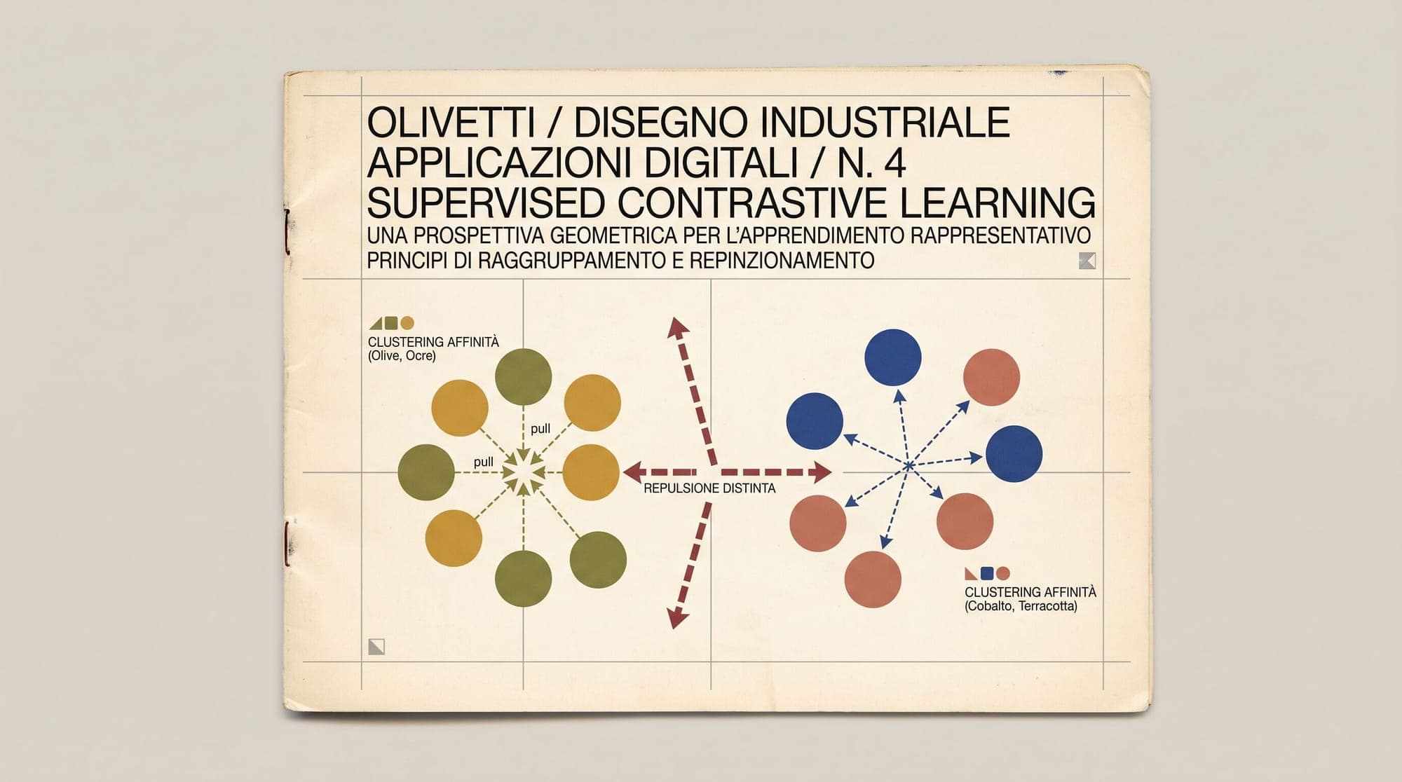
In 2020, researchers at Google Brain and MIT introduced Supervised Contrastive Learning (SupCon). By bridging self-supervised batch contrastive estimation and fully supervised classification, SupCon extends the multi-class InfoNCE objective to leverage label information. Instead of contrasting a single positive view against all other batch elements, SupCon pulls all augmented samples belonging to the same class together on a unit hypersphere while pushing samples from differing classes apart. The resulting representation space achieves greater class separation, improved transferability, and heightened resilience to data distribution shifts.

The Limitations of Standard Cross-Entropy

In a standard classification pipeline, an encoder network $f(\cdot)$ maps an input $x$ to an intermediate representation $h = f(x) \in \mathbb{R}^{d}$. A linear classification layer parameterized by weight vectors $W = [w_1, w_2, \dots, w_C]^\top$ computes class logits $z_c = w_c^\top h$, which are normalized via the softmax function:

$$P(y = c \mid x) = \frac{\exp(w_c^\top h / \tau)}{\sum_{j=1}^C \exp(w_j^\top h / \tau)}$$

The cross-entropy loss for a ground-truth label $y$ is defined as:

$$\mathcal{L}_{\text{CE}} = -\log \frac{\exp(w_y^\top h / \tau)}{\sum_{j=1}^C \exp(w_j^\top h / \tau)}$$

While mathematically straightforward, this objective introduces three fundamental geometric constraints:

1. Hyperplane Competition Over Representation Geometry: Cross-entropy measures the alignment of intermediate features $h$ against static linear weight vectors $w_c$. Once a feature vector crosses the decision hyperplane with sufficient confidence, the gradient magnitude diminishes rapidly. The loss does not penalize representations for clustering tightly against the decision boundary, leaving the latent space susceptible to out-of-distribution (OOD) vulnerability.
2. Independent Augmentation Processing: When input augmentations (e.g., cropping, color jittering, masking) are applied during training, cross-entropy penalizes each view independently against the one-hot target vector. It enforces no explicit constraint that two distinct augmentations of the same underlying image or text sequence must yield adjacent embeddings in latent space.
3. Lack of Intrinsic Margin Regularization: Because cross-entropy optimizes probability distributions rather than distance metrics in feature space, it does not guarantee that the intra-class variance remains smaller than inter-class distances.

Self-Supervised Contrastive Mechanics: The Baseline InfoNCE

To eliminate the need for manual labels, self-supervised representation frameworks such as SimCLR and MoCo introduced batch contrastive objectives based on InfoNCE.

For a multiview batch of $2N$ samples generated by applying two random augmentations to $N$ unlabelled inputs, let $i \in I \equiv \{1, \dots, 2N\}$ be the index of an arbitrary anchor sample. Let $j(i)$ denote the index of the corresponding alternate augmentation (the single positive). The normalized latent representations $z_i = g(h_i) / \|g(h_i)\|_2$ lie on the unit hypersphere $\mathcal{S}^{d-1}$, where $g(\cdot)$ is a non-linear projection head.

The self-supervised InfoNCE (NT-Xent) loss is formulated as:

$$\mathcal{L}^{\text{self}} = \sum_{i \in I} \mathcal{L}_i^{\text{self}} = -\sum_{i \in I} \log \frac{\exp(z_i \cdot z_{j(i)} / \tau)}{\sum_{a \in A(i)} \exp(z_i \cdot z_a / \tau)}$$

Where $A(i) \equiv I \setminus \{i\}$, and $\tau > 0$ represents a scalar temperature hyperparameter.

While self-supervised InfoNCE successfully forces representations to be invariant to data augmentations, it suffers from false negatives when applied to structured domains. In any mini-batch containing multiple unlabelled instances of the same semantic class (e.g., two distinct images of dogs), the self-supervised loss actively repels their embeddings, creating artificial semantic dispersion.

The Supervised Contrastive Loss Formulation

Supervised Contrastive Learning resolves the false negative bottleneck by integrating label metadata directly into the multi-view contrastive denominator. In a batch of $N$ labeled pairs $(x_k, y_k)$, data augmentation generates $2N$ views. For each anchor $i$, the index set of all positive samples sharing the same label is defined as:

$$P(i) \equiv \{p \in A(i) : y_p = y_i\}$$

Where $|P(i)|$ is the total cardinality of positives for anchor $i$ in the batch.

Khosla et al. analyzed two mathematical extensions of InfoNCE to multi-positive sets: placing the summation inside the logarithm ($\mathcal{L}_{\text{in}}^{\text{sup}}$) versus outside the logarithm ($\mathcal{L}_{\text{out}}^{\text{sup}}$).

Self-Supervised InfoNCE:
Anchor (i)  <--- Pull --->  Augmented View j(i)
Anchor (i)  <=== Push ===>  All Other (2N - 2) Batch Samples

Supervised Contrastive (SupCon):
Anchor (i)  <--- Pull --->  All Samples with Label y_p == y_i (Augmentations + Distinct Class Instances)
Anchor (i)  <=== Push ===>  All Samples with Label y_a != y_i

The Optimal Loss: $\mathcal{L}_{\text{out}}^{\text{sup}}$

The benchmark SupCon loss places the summation over positive pairs outside the logarithmic operation:

$$\mathcal{L}_{\text{out}}^{\text{sup}} = \sum_{i \in I} \frac{-1}{|P(i)|} \sum_{p \in P(i)} \log \frac{\exp(z_i \cdot z_p / \tau)}{\sum_{a \in A(i)} \exp(z_i \cdot z_a / \tau)}$$

Placing the summation outside the logarithm provides critical optimization properties:

• Uniform Gradient Distribution: Under $\mathcal{L}_{\text{out}}^{\text{sup}}$, every positive pair $(i, p)$ contributes an independent gradient term. The model is forced to pull all intra-class samples closer simultaneously.
• Avoidance of Positive Saturation: In contrast, the formulation $\mathcal{L}_{\text{in}}^{\text{sup}} = -\sum_i \log \left( \frac{1}{|P(i)|} \sum_{p \in P(i)} \frac{\exp(z_i \cdot z_p / \tau)}{\sum_a \exp(z_i \cdot z_a / \tau)} \right)$ allows a single highly aligned positive pair ($z_i \cdot z_p \approx 1$) to dominate the inner sum. Once one positive is satisfied, the loss gradient for remaining difficult intra-class positives collapses toward zero.

Hyperspherical Geometry: Alignment, Uniformity, and Gradients

To understand why SupCon produces superior feature representations, one must inspect the loss dynamics on the unit hypersphere $\mathcal{S}^{d-1}$. As formalized by Wang and Isola (2020), optimal representation learning balances two geometric properties:

1. Alignment: Features from semantically related samples should map to nearby points on the hypersphere:

$$\mathcal{L}_{\text{align}} \triangleq \mathbb{E}_{(x, x^+) \sim p_{\text{pos}}} [\|z - z^+\|_2^2]$$

1. Uniformity: The global distribution of feature vectors should preserve maximal information by distributing uniformly across the unit hypersphere:

$$\mathcal{L}_{\text{uniform}} \triangleq \log \mathbb{E}_{x, y \stackrel{i.i.d.}{\sim} p_{\text{data}}} \left[ \exp(-2 \|z_x - z_y\|_2^2) \right]$$

SupCon achieves supervised alignment and uniformity simultaneously. Positive pairs within the same class contract toward shared cluster centroids (alignment), while the contrastive denominator forces distinct class clusters to repel each other, maximizing the angular distance between class centroids across the hypersphere (uniformity).

Gradient Dynamics and Hard-Sample Mining

The gradient of $\mathcal{L}_{\text{out}}^{\text{sup}}$ with respect to the anchor embedding $z_i$ reveals implicit hard-sample mining:

$$\frac{\partial \mathcal{L}_{\text{out}}^{\text{sup}}}{\partial z_i} = \frac{1}{\tau} \sum_{p \in P(i)} \left( P_{ip} - \frac{1}{|P(i)|} \right) z_p + \frac{1}{\tau} \sum_{n \in N(i)} P_{in} z_n$$

Where $N(i) \equiv \{n \in A(i) : y_n \neq y_i\}$ represents the set of negative samples, and $P_{ia}$ is the softmax probability:

$$P_{ia} = \frac{\exp(z_i \cdot z_a / \tau)}{\sum_{b \in A(i)} \exp(z_i \cdot z_b / \tau)}$$

This gradient structure yields two operational dynamics:

• Hard Negative Repulsion: If a negative sample $n$ from a different class is located close to anchor $i$ in cosine space ($z_i \cdot z_n \gg 0$), $P_{in}$ becomes large, exerting an aggressive repulsive force along vector $z_n$.
• Hard Positive Attraction: If a positive sample $p$ from the same class has poor alignment ($z_i \cdot z_p \ll 1$), $P_{ip}$ is small, making the negative coefficient $(P_{ip} - 1/|P(i)|)$ large and pulling $z_i$ sharply toward $z_p$.
• Temperature Scaling ($\tau$): Lower values of $\tau$ sharpen the probability distribution, heavily penalizing the most difficult violations (hardest negatives and hardest positives), whereas larger $\tau$ values smooth the gradient across all batch members.

Two-Stage Training Architecture

Deploying Supervised Contrastive Learning in production follows a two-stage decoupled training protocol:

Stage 1: Representation Pre-Training (SupCon)
Input x ---> Augmentations [x_1, x_2] ---> Base Encoder f(·) ---> Representation h ---> Projection Head g(·) ---> Latent z on Sphere ---> SupCon Loss

Stage 2: Classifier Training (Linear Probe)
Input x ---> Base Encoder f(·) (Frozen) ---> Representation h ---> Linear Classifier W ---> Cross-Entropy Loss ---> Predictions

Stage 1: Feature Learning via Projection Head

The input $x$ passes through data augmentation pipelines to create multiview pairs. The base encoder $f(\cdot)$ extracts hidden vectors $h = f(x) \in \mathbb{R}^{d_{\text{enc}}}$. A non-linear projection head $g(\cdot)$ (typically a 2-layer MLP with ReLU activation and hidden dimension 2048) maps $h$ to a lower-dimensional latent space $z = g(h) \in \mathbb{R}^{d_{\text{proj}}}$. The vectors $z$ are normalized to unit length, and the entire network is trained end-to-end using $\mathcal{L}_{\text{out}}^{\text{sup}}$.

Stage 2: Linear Classifier Readout

Once representation training converges, the projection head $g(\cdot)$ is discarded. The base encoder $f(\cdot)$ is frozen. A standard linear classifier layer $W \in \mathbb{R}^{C \times d_{\text{enc}}}$ is appended directly to the base representations $h$. The linear layer is trained with standard cross-entropy loss while keeping encoder weights fixed.

Retaining the base representation $h$ rather than the projection output $z$ is essential. The non-linear projection head $g(\cdot)$ discards information that is invariant under the specific contrastive loss (such as color distribution or high-frequency textures), while the intermediate representation $h$ preserves generalizable semantic features.

Empirical Performance and Robustness

Rigorous benchmarking across standard vision and multimodal datasets demonstrates distinct advantages over end-to-end cross-entropy:

| Metric / Benchmark | Cross-Entropy Baseline | Supervised Contrastive (SupCon) | Delta | | :--- | :--- | :--- | :--- | | ImageNet Top-1 Accuracy (ResNet-50) | 76.5% | 78.7% | +2.2% | | ImageNet Top-1 Accuracy (ResNet-200) | 79.9% | 81.4% | +1.5% | | ImageNet-C Mean Corruption Error (mCE) | 51.5 (lower is better) | 44.1 | -7.4 mCE | | Hyperparameter Sensitivity ($\Delta$ LR) | High (diverges easily) | Low (stable across 10x range) | Robust | | Label Noise Robustness (20% corrupted) | Significant degradation | High retention of top-1 accuracy | Robust |

Robustness to Corruptions and Out-of-Distribution Data

Because SupCon explicitly maximizes margin boundaries between class clusters on the hypersphere, the resulting representations exhibit substantially lower error rates on corrupted benchmark distributions (e.g., ImageNet-C, ImageNet-R). When inputs undergo Gaussian blur, compression artifacts, or weather-related noise, their embeddings remain within their respective class hyperspherical clusters rather than drifting across narrow linear classification planes.

Modern Applications: LLMs, Embeddings, and Alignment

While originally evaluated on vision encoders, the principles of Supervised Contrastive Learning underpin modern architectures across the AI stack:

1. Dense Retrieval and Bi-Encoder Embedding Models: Modern text embedding architectures (such as BGE, E5, and Contriever) rely on multi-positive supervised contrastive objectives during fine-tuning. In dense retrieval, a single query often possesses multiple valid passage matches (positives) within a corpus; SupCon allows all relevant passages to pull toward the query embedding while repelling in-batch and hard negatives.
2. AI Guardrails and Intent Classification: Embedding models trained with SupCon serve as the classification backbone for safety guardrails and prompt routing. Grouping adversarial prompts, jailbreaks, and benign user inputs into structured clusters enables reliable threshold-based Out-of-Distribution (OOD) detection via cosine similarity or Mahalanobis distance.
3. Multimodal Alignment (CLIP and SigLIP): Vision-language foundation models like CLIP and SigLIP adapt contrastive mechanics to align paired image-text embeddings across a shared latent space, leveraging multi-positive formulations when scaling to web-scraped datasets with overlapping semantic tags.

Sources

• Khosla, P., Teterwak, P., Wang, C., Sarna, A., Tian, Y., Isola, P., Maschinot, A., Liu, C., & Krishnan, D. (2020). Supervised Contrastive Learning. Advances in Neural Information Processing Systems (NeurIPS 2020).
• Chen, T., Kornblith, S., Norouzi, M., & Hinton, G. (2020). A Simple Framework for Contrastive Learning of Visual Representations (SimCLR). International Conference on Machine Learning (ICML 2020).
• Wang, T., & Isola, P. (2020). Understanding Contrastive Representation Learning through Alignment and Uniformity on the Hypersphere. International Conference on Machine Learning (ICML 2020).
• He, K., Fan, H., Wu, Y., Xie, S., & Girshick, R. (2020). Momentum Contrast for Unsupervised Visual Representation Learning (MoCo). CVPR 2020.
• Radford, A., Kim, J. W., Hallacy, C., Ramesh, A., Goh, G., Agarwal, S., Sastry, G., Askell, A., Mishkin, P., Clark, J., Krueger, G., & Sutskever, I. (2021). Learning Transferable Visual Models From Natural Language Supervision (CLIP). ICML 2021.
• Zhai, X., Mustafa, B., Kolesnikov, A., & Beyer, L. (2023). Sigmoid Loss for Language Image Pre-Training (SigLIP). ICCV 2023.