Structured State Space Models and Mamba: Mathematical Foundations, Continuous Discretization, and Hardware-Aware Associative Scans

The dominant architectural paradigm in modern deep learning relies on Transformer multi-head self-attention. While self-attention achieves expressive sequence modeling by enabling every token to directly route information to and from every preceding token, it introduces steep computational overheads: training and prefill compute scale quadratically with sequence length (O(L^2)), and autoregressive inference requires an uncompressed Key-Value (KV) cache that scales linearly with sequence length (O(L)) in GPU memory per active sequence.

Recurrent Neural Networks (RNNs) historically offered an alternative: maintaining a constant-size hidden state (O(1) memory footprint during generation) with O(1) step computation. However, classical RNNs suffered from sequential training dependencies that prevented efficient parallelization on modern GPU clusters, along with vanishing or exploding gradients over long contexts.

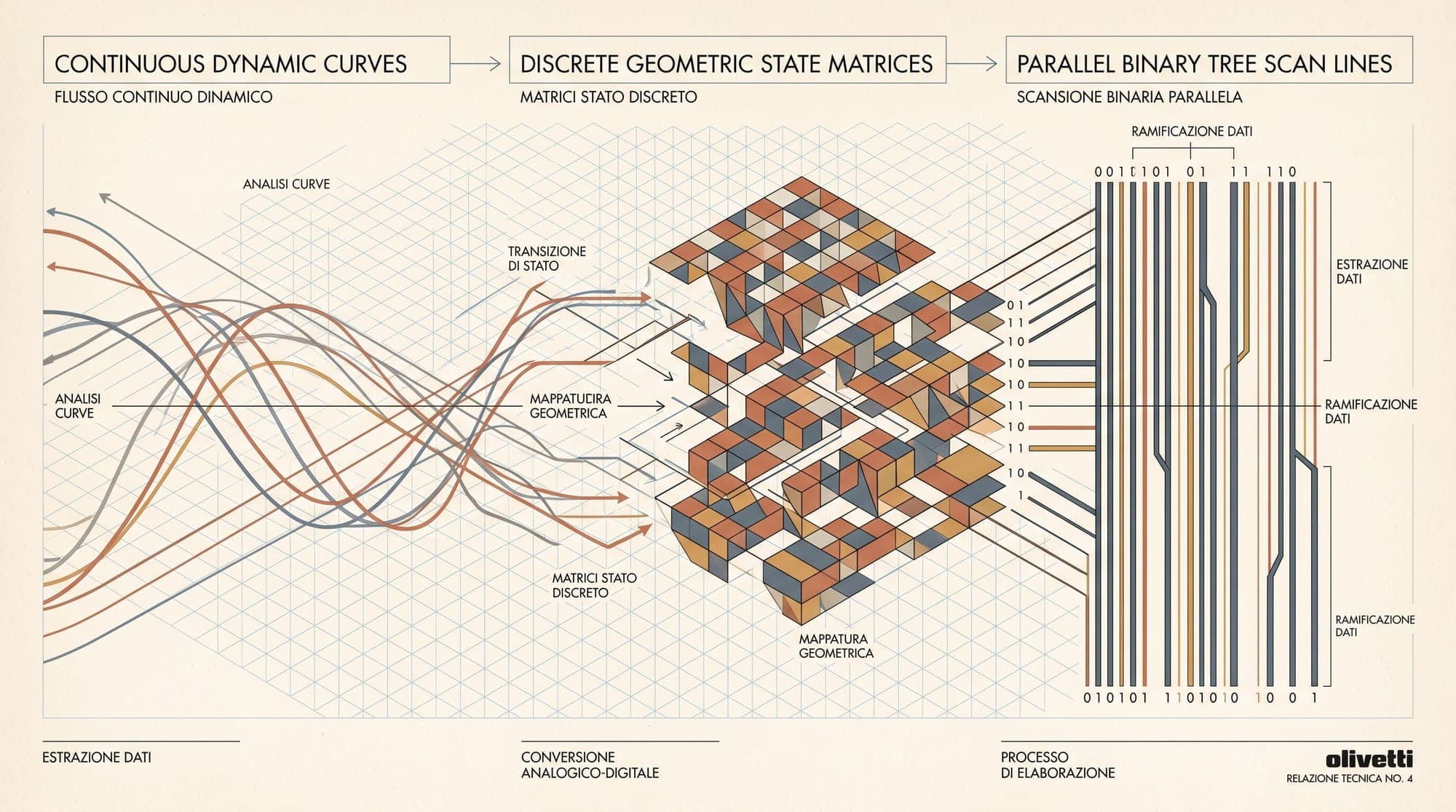
Structured State Space Sequence Models (SSMs), culminating in architectures like S4 and Mamba (S6), resolve this tension. By framing sequence modeling through the lens of continuous-time dynamical systems, discretizing differential equations with rigorous mathematical structures (such as HiPPO matrices), and executing time-varying recurrences via hardware-aware parallel associative scans in GPU SRAM, modern SSMs achieve linear-time sequence processing (O(L)) during training and constant-time (O(1)) autoregressive inference without an expanding KV cache.

Continuous-Time Dynamical Systems

At its mathematical foundation, a linear continuous-time state space model maps a continuous 1D input signal x(t) to an output signal y(t) through an N-dimensional latent state representation h(t). The system is governed by a pair of coupled linear differential equations:

h'(t) = A h(t) + B x(t)
y(t)  = C h(t) + D x(t)

In this formulation:

h(t) is an N-dimensional hidden state vector representing the memory of the dynamical system.
x(t) is the continuous scalar input at time t (extended across D independent channels in multidimensional architectures).
A is the N x N transition matrix (system dynamics operator) that controls the decay, oscillation, and propagation of hidden states.
B is the N x 1 input projection matrix that injects the scalar input into the N-dimensional state space.
C is the 1 x N output projection matrix that decodes the latent state into the scalar output.
D is a scalar direct feedthrough (skip-connection) parameter, often omitted or parameterized as a simple residual connection.

The continuous formulation provides two desirable properties: resolution invariance (the model can process signals sampled at arbitrary or variable frequencies) and analytical tractability over infinite continuous domains.

Discretization Mechanics: Zero-Order Hold and Bilinear Transforms

Digital computers operate on discrete sequences of tokens rather than continuous signals. To apply continuous state space models to discrete token sequences (x_0, x_1, ..., x_{L-1}), the continuous differential equations must be discretized relative to a positive step size parameter Delta > 0.

The standard discretization method in state space sequence models is the Zero-Order Hold (ZOH) assumption, which posits that the input signal x(t) remains constant over the discrete interval [kDelta, (k+1)Delta).

Integrating the continuous ODE over the interval t in [kDelta, (k+1)Delta) yields the exact analytical transition:

h_k = exp(Delta * A) h_{k-1} + (int_0^Delta exp(tau * A) d tau) B x_k

Evaluating the integral produces the discrete transition matrices A_bar and B_bar:

A_bar = exp(Delta * A)
B_bar = (Delta * A)^(-1) * (exp(Delta * A) - I) * (Delta * B)

The resulting discrete-time state space model operates as a recurrent update:

h_k = A_bar * h_{k-1} + B_bar * x_k
y_k = C * h_k + D * x_k

An alternative discretization method is the Bilinear (Tustin's) transform, derived from trapezoidal numerical integration:

A_bar = (I - (Delta / 2) * A)^(-1) * (I + (Delta / 2) * A)
B_bar = (I - (Delta / 2) * A)^(-1) * (Delta * B)

The step size Delta acts as a dynamic timescale parameter:

When Delta is small, the transition matrix A_bar approaches the identity matrix (exp(Delta * A) -> I), causing the hidden state to retain its existing memory while ignoring new inputs (B_bar -> 0).
When Delta is large, A_bar decays historical states rapidly, prioritizing the instantaneous current input x_k.

Structured State Spaces (S4) and the HiPPO Memory Framework

When the transition matrix A is initialized randomly from standard Gaussian or uniform distributions, discrete recurrences collapse: hidden states either explode exponentially or vanish completely when unrolled across thousands of sequential steps.

The Structured State Space (S4) architecture developed by Gu, Goel, and Ré (2021) solved this memory decay problem by applying the High-order Polynomial Projection Operators (HiPPO) framework established by Gu et al. (2020).

HiPPO proves that maintaining an optimal online polynomial approximation of a continuous signal history against an exponentially shifted Legendre polynomial basis requires a specific transition matrix structure:

A_{n, k} = -sqrt(2n + 1) * sqrt(2k + 1)   if n > k
A_{n, k} = -(n + 1)                       if n = k
A_{n, k} = 0                              if n < k

When initialized with this HiPPO matrix, the latent state h(t) acts as a compressed spectral projection of the entire continuous history of input x(<=t), eliminating the vanishing gradient problem across long context windows.

For Linear Time-Invariant (LTI) systems, where matrices A_bar, B_bar, and C remain strictly constant across all time steps, the discrete recurrence can be unrolled explicitly:

y_0 = C * B_bar * x_0
y_1 = C * A_bar * B_bar * x_0 + C * B_bar * x_1
y_2 = C * A_bar^2 * B_bar * x_0 + C * A_bar * B_bar * x_1 + C * B_bar * x_2
...
y_k = sum_{j=0}^k (C * A_bar^(k-j) * B_bar) * x_j

This unrolled summation is mathematically equivalent to a 1D non-causal circular convolution:

y = x * K_bar
K_bar = (C * B_bar, C * A_bar * B_bar, C * A_bar^2 * B_bar, ..., C * A_bar^(L-1) * B_bar)

This dual representation gave S4 two simultaneous operating modes:

Training mode: The convolutional kernel K_bar is computed once, and the full output sequence y is generated in parallel across sequence length L via the Fast Fourier Transform (FFT) in O(L log L) time.
Inference mode: The model switches to the recurrent representation (h_k = A_bar * h_{k-1} + B_bar * x_k), generating each token in O(1) step compute without caching historical activations.

Structured State Space Memory Hierarchy and Associative Scan

The Linear Time-Invariance Bottleneck and the Selective State Space (S6)

While S4 achieved high throughput and long-context scaling on benchmarks like Long Range Arena, LTI state space models suffered from a fundamental representational limitation: they could not perform content-based reasoning.

In a strictly Linear Time-Invariant system, the convolution kernel K_bar is static and identical regardless of the input tokens. An LTI model applies the exact same weight decay and receptive field to every token, preventing it from performing basic language tasks such as:

Selective Copying: Memorizing a specific key token encountered early in a prompt and reproducing it hundreds of tokens later.
Associative Recall: Dynamically linking arbitrary keys to values and retrieving the value upon encountering the key.
Content-Aware Filtering: Adjusting the timescale Delta to ignore irrelevant filler tokens while concentrating capacity on semantically dense tokens.

To solve this, Gu and Dao (2023) introduced Mamba (the S6 model), which replaces the fixed LTI formulation with a Linear Time-Varying (LTV) Selective State Space mechanism.

In S6, the matrices B, C, and the discretization step size Delta are parameterized as data-dependent linear projections of the instantaneous input token x_t:

B_t     = Linear_B(x_t)
C_t     = Linear_C(x_t)
Delta_t = softplus(Linear_Delta(x_t) + Parameter_bias)

Because Delta_t, B_t, and C_t change dynamically with every token x_t:

The discrete transition matrix becomes token-dependent: A_bar_t = exp(Delta_t * A).
The discrete input matrix becomes token-dependent: B_bar_t = (Delta_t * A)^(-1) * (exp(Delta_t * A) - I) * (Delta_t * B_t).

By making Delta_t input-dependent, Mamba can selectively reset its memory (by increasing Delta_t to erase past state) or protect its memory indefinitely (by driving Delta_t toward zero so A_bar_t becomes identity).

However, introducing time-varying matrices breaks shift invariance. The system can no longer be unrolled into a single stationary convolution kernel K_bar, which prevents the use of Fast Fourier Transforms (FFT) for parallel training.

Hardware-Aware Parallel Associative Scan

To train a time-varying recurrence efficiently without falling back to slow sequential loops on GPUs, Mamba leverages the Parallel Associative Scan algorithm, rooted in prefix sum principles established by Blelloch (1990).

The first-order linear recurrence:

h_t = A_bar_t * h_{t-1} + B_bar_t * x_t

can be formalized as a binary associative operator acting on pairs of transition elements (A_bar_t, u_t), where u_t = B_bar_t * x_t.

Defining the binary composition operator:

(A_i, u_i) * (A_j, u_j) = (A_j * A_i, A_j * u_i + u_j)

This operator satisfies the associative property:

((A_1, u_1) * (A_2, u_2)) * (A_3, u_3) = (A_1, u_1) * ((A_2, u_2) * (A_3, u_3))

Because the operator is strictly associative, all prefix evaluations h_0, h_1, ..., h_{L-1} can be computed using a parallel tree reduction (up-sweep and down-sweep phases) in O(log L) parallel step depth and O(L) total work across GPU worker threads.

The GPU Memory Hierarchy and Kernel Fusion

The remaining architectural bottleneck is physical memory bandwidth. In standard PyTorch or naive CUDA implementations, materializing the full 4D state tensor (Batch B, Sequence Length L, Model Dimension D, State Dimension N) in GPU High Bandwidth Memory (HBM) requires immense memory traffic:

For a sequence of length L = 16,384, dimension D = 2,048, and state size N = 16, a single forward pass would materialize:

Memory = 16,384 * 2,048 * 16 * 2 bytes (FP16) = 1.07 GB per sequence

Reading and writing this intermediate state tensor to HBM at every layer completely bottlenecks modern GPUs, which are memory-bandwidth bound rather than compute bound.

Mamba circumvents this via a custom GPU kernel fusion strategy:

Inputs x, Delta, B, and C are loaded directly from HBM into fast on-chip SRAM (Static RAM / Shared Memory).
Continuous discretization (computing A_bar_t and B_bar_t) is computed in-flight within SRAM registers.
The parallel associative scan is executed entirely inside on-chip SRAM across thread blocks.
The hidden state h_t is multiplied by C_t within SRAM to produce the final output y_t.
Only the final output y_t (of shape B x L x D) is written back to HBM.

By keeping the expanded N-dimensional state strictly inside GPU SRAM, Mamba eliminates intermediate HBM memory round-trips, achieving training throughput comparable to or exceeding FlashAttention-2.

Structural Comparison: Transformers vs. S4 vs. Mamba

The architectural trade-offs across attention and state space paradigms can be evaluated across their theoretical complexity and operational profiles:

Multi-Head Self-Attention (Transformers):
Training Compute Complexity: O(L^2) per layer.
Training Parallelism: Fully parallel (matrix multiplications).
Inference Step Time: O(L) compute per step as context expands.
Inference Memory Footprint: O(L) KV cache per sequence in HBM.
In-Context Associative Recall: Exact (non-parametric lookup across all historical tokens).
Structured State Spaces (S4 / LTI):
Training Compute Complexity: O(L log L) per layer via FFT convolution.
Training Parallelism: Fully parallel (FFT).
Inference Step Time: O(1) constant per step.
Inference Memory Footprint: O(1) fixed state size (D x N).
In-Context Associative Recall: Poor (fixed linear time-invariant filtering).
Selective State Spaces (Mamba / S6):
Training Compute Complexity: O(L) per layer via fused parallel associative scan.
Training Parallelism: Parallel tree scan across sequence dimension.
Inference Step Time: O(1) constant per step.
Inference Memory Footprint: O(1) fixed state size (D x N).
In-Context Associative Recall: High (dynamic token-dependent gating and memory routing).

Information-Theoretic Trade-Offs and Failure Modes

While Mamba and selective SSMs provide linear scaling and constant-memory inference, their fixed-size hidden state (D x N) imposes theoretical boundaries compared to Transformers:

State Compression Limits: A Transformer stores the uncompressed representations of all previous tokens in its KV cache. In contrast, an SSM compresses an arbitrarily long sequence into a fixed vector space of dimension D x N. When a task requires memorizing a massive set of uncorrelated key-value pairs (e.g. dense long-context needle retrieval with dozens of conflicting keys), the fixed state capacity eventually suffers from information loss.
Complex Multi-Hop Pointer Tracing: Transformers can execute arbitrary multi-hop graph traversals across tokens in a single forward pass by stacking attention layers. In an SSM, routing information between non-adjacent tokens requires either multiple recurrent steps or layer-stack propagation.
Quantization Dynamics: Because the hidden state h_t accumulates recurrent products of A_bar_t over time, low-precision quantization (e.g. INT4 or FP4) of recurrent state updates requires tighter scale tracking to prevent numerical drift across long sequences.

State Space Duality and Mamba-2

The theoretical evolution of state spaces reached a further milestone with Structured State Space Duality (SSD), introduced in Mamba-2 by Dao and Gu (2024).

SSD proves an exact algebraic equivalence between 1D structured state space models and masked linear attention variants with structured scalar decay matrices:

Y = (L * (Q * K^T)) * V

where L is a 1-semiseparable matrix representing the exponential state space decay.

By formulating the state space recurrence as block-diagonal matrix multiplications, Mamba-2 executes on Tensor Cores using standard matrix multiplication hardware (GEMMs), increasing training throughput while unifying the mathematical formulations of attention, linear attention, and continuous state spaces into a single framework.

Sources

Efficiently Modeling Long Sequences with Structured State Spaces (S4) - Gu, Goel, and Ré (NeurIPS 2021)
Mamba: Linear-Time Sequence Modeling with Selective State Spaces - Gu and Dao (2023)
HiPPO: Recurrent Memory with Optimal Polynomial Projections - Gu, Dao, Ermon, Rudra, and Ré (NeurIPS 2020)
Simplified State Space Layers for Sequence Modeling (S5) - Smith, Warrington, and Linderman (ICLR 2023)
Transformers are SSMs: Generalized Models and Efficient Algorithms Through Structured State Space Duality - Dao and Gu (ICML 2024)
Prefix Sums and Their Applications - Guy E. Blelloch (Technical Report CMU-CS-90-190, 1990)