Post-Training Quantization (PTQ): Mathematical Foundations of Optimal Brain Surgeon, GPTQ Hessian Inversion, AWQ Salient Scaling, and SmoothQuant Outlier Migration

Serving modern large language models at scale requires addressing severe hardware constraints. In autoregressive generation, decoding is fundamentally bounded by memory bandwidth rather than floating-point computation throughput. Each generated token requires reading every parameter from High Bandwidth Memory (HBM) into SRAM to perform matrix-vector multiplications. For a 70-billion parameter model in FP16 or BF16 precision, a single forward pass transfers 140 gigabytes of weights. On an NVIDIA H100 GPU with 3.35 terabytes per second of memory bandwidth, transferring these weights establishes a theoretical limit of roughly 24 tokens per second for batch size 1.

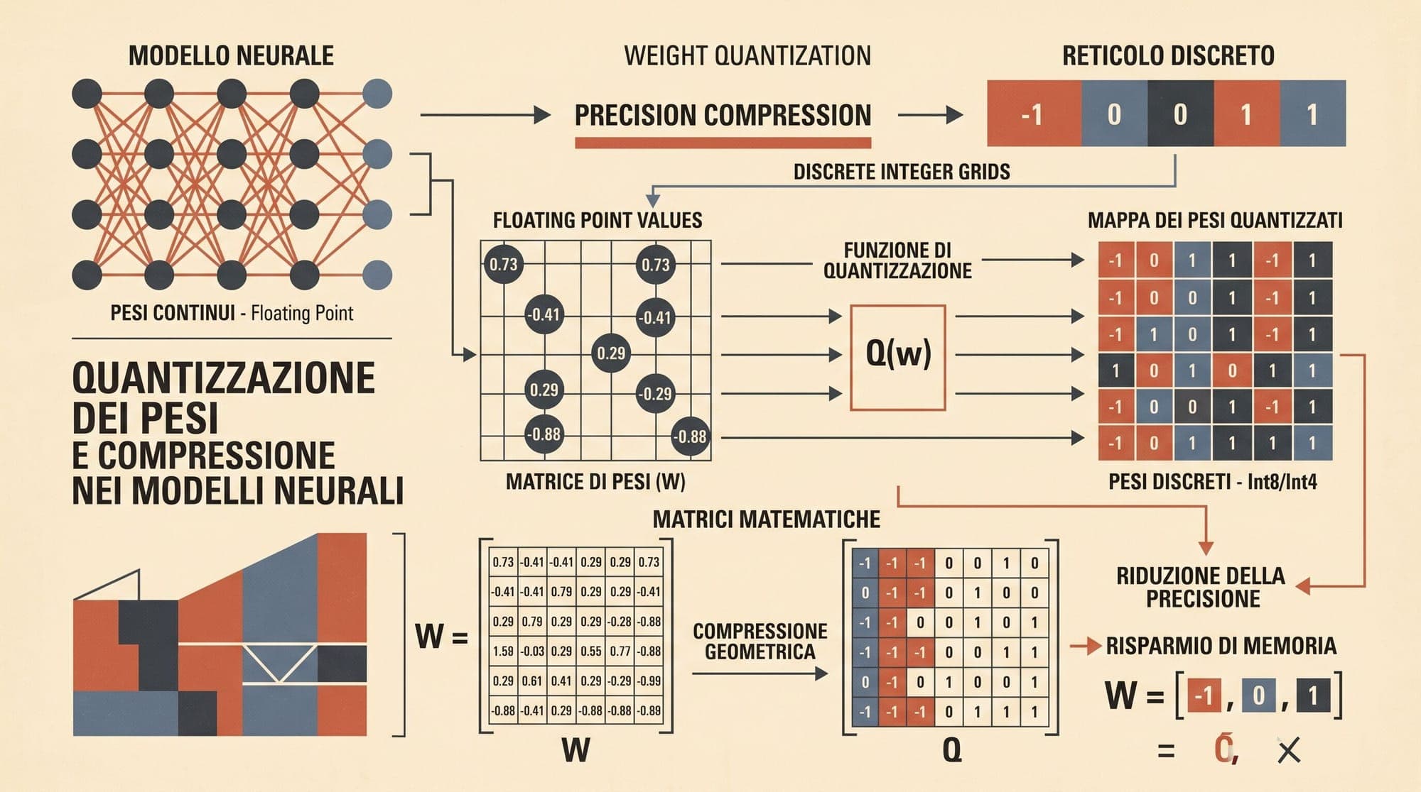
Post-Training Quantization (PTQ) addresses this memory wall by mapping high-precision floating-point parameters (FP16, BF16, or FP32) to low-bitwidth discrete representations (such as INT8, INT4, or FP8) without requiring extensive end-to-end retraining. Achieving low-bit quantization without degrading model perplexity requires rigorous mathematical compensation techniques.

Fundamentals of Uniform and Affine Quantization

The standard quantization operation maps continuous real-valued numbers into discrete integer bins.

Uniform Affine Quantization

Uniform affine (asymmetric) quantization maps a real-valued interval $[x_{\min}, x_{\max}]$ to an unsigned $b$-bit integer range $[0, 2^b - 1]$ through a positive scale factor $S$ and an integer zero-point offset $Z$:

$$S = \frac{x_{\max} - x_{\min}}{2^b - 1}$$

$$Z = \text{round}\left(-\frac{x_{\min}}{S}\right)$$

The quantization function $Q(x)$ applies scaling, rounding, offset addition, and clamping:

$$Q(x) = \text{clip}\left(\text{round}\left(\frac{x}{S}\right) + Z, 0, 2^b - 1\right)$$

The corresponding dequantization function reconstructs an approximate real value $\hat{x}$:

$$\hat{x} = S \cdot (Q(x) - Z)$$

Symmetric Quantization

When data distributions are roughly centered around zero, symmetric quantization simplifies the mapping by setting the zero-point $Z = 0$. For signed $b$-bit integers spanning $[-2^{b-1}, 2^{b-1} - 1]$, the scale factor is derived from the maximum absolute value:

$$S = \frac{\max(|x|)}{2^{b-1} - 1}$$

$$Q(x) = \text{clip}\left(\text{round}\left(\frac{x}{S}\right), -2^{b-1}, 2^{b-1} - 1\right)$$

$$\hat{x} = S \cdot Q(x)$$

Symmetric quantization removes the overhead of subtracting zero points during matrix multiplication, enabling hardware integer Tensor Cores to execute integer multiply-accumulate (IMAC) operations directly.

Quantization Granularity

Quantization operates at various structural granularities:

• Per-tensor quantization: A single scale factor $S$ is shared across an entire weight tensor or activation matrix. This minimizes metadata overhead but suffers when activation or weight distributions vary widely across channels.
• Per-channel (per-column / per-row) quantization: An independent scale factor is assigned to each output channel (row) of a weight matrix $W \in \mathbb{R}^{d_{\text{out}} \times d_{\text{in}}}$. This captures inter-channel variance without altering matrix multiplication hardware execution patterns.
• Group-wise (sub-channel) quantization: Consecutive elements along the input channel dimension are partitioned into groups of size $g$ (typically $g \in \{32, 64, 128\}$), with an independent scale factor per group. Group-wise quantization limits the propagation of local outlier values, substantially improving accuracy at 3-bit and 4-bit precisions at the cost of additional scale parameters.

Optimal Brain Surgeon: Second-Order Error Minimization

Rounding weights to the nearest discrete integer independently (Round-To-Nearest, or RTN) causes quantization errors to compound across layers. To minimize the output distortion of a linear layer $Y = W X$, post-training quantization seeks to minimize the layer-wise Mean Squared Error (MSE):

$$\mathcal{L} = \frac{1}{2} \| W X - \hat{W} X \|_2^2 = \frac{1}{2} \text{Tr}\left((W - \hat{W}) X X^T (W - \hat{W})^T\right)$$

Here, $W \in \mathbb{R}^{d_{\text{out}} \times d_{\text{in}}}$ denotes the original unquantized weight matrix, $\hat{W}$ represents the quantized weight matrix, and $X \in \mathbb{R}^{d_{\text{in}} \times N}$ represents the layer inputs collected from a small calibration dataset of unlabelled tokens.

The optimization can be decoupled across each row $w \in \mathbb{R}^{1 \times d_{\text{in}}}$ of $W$:

$$\mathcal{L}(w) = \frac{1}{2} (w - \hat{w}) H (w - \hat{w})^T$$

where the Hessian matrix $H \in \mathbb{R}^{d_{\text{in}} \times d_{\text{in}}}$ of second-order derivatives is given by:

$$H = \nabla_w^2 \mathcal{L} = 2 X X^T$$

Applying a second-order Taylor expansion around the unquantized optimal weight vector $w$:

$$\Delta \mathcal{L} = \mathcal{L}(w + \Delta w) - \mathcal{L}(w) = \nabla_w \mathcal{L}^T \Delta w + \frac{1}{2} \Delta w^T H \Delta w$$

Because the pre-trained weights $w$ represent an unconstrained local minimum of the layer loss, the first-order gradient vanishes: $\nabla_w \mathcal{L} = 0$. The change in error simplifies to:

$$\Delta \mathcal{L} \approx \frac{1}{2} \Delta w^T H \Delta w$$

In the classical Optimal Brain Surgeon (OBS) formulation, when a specific weight component $w_q$ is quantized to $\hat{w}_q$ (enforcing the constraint $e_q^T \Delta w = \hat{w}_q - w_q$), the remaining unquantized weights are adjusted to compensate for the perturbation. Solving the constrained optimization problem via Lagrange multipliers yields the OBS weight update rule:

$$\Delta w = - \frac{w_q - \hat{w}_q}{[H^{-1}]_{qq}} H^{-1}_{:, q}$$

The resulting increase in reconstruction error is:

$$\Delta \mathcal{L} = \frac{1}{2} \frac{(w_q - \hat{w}_q)^2}{[H^{-1}]_{qq}}$$

Here, $H^{-1}_{:, q}$ denotes the $q$-th column of the inverse Hessian matrix, and $[H^{-1}]_{qq}$ is its $q$-th diagonal element.

GPTQ: Efficient Second-Order Quantization at Scale

Direct application of Optimal Brain Surgeon to modern transformers is computationally intractable. For an input dimension $d_{\text{in}} = 8192$, computing and updating the full inverse Hessian matrix for each scalar weight parameter requires $O(d^4)$ operations, requiring hundreds of GPU hours per layer.

The GPTQ algorithm optimizes this process through three primary innovations:

1. Arbitrary Quantization Ordering

While classical OBS greedily selects the weight that minimizes $\Delta \mathcal{L}$ at each step, GPTQ demonstrates that quantizing weights in a fixed, column-by-column order across all rows yields nearly identical perplexity. Fixing the column order allows the algorithm to share the inverse Hessian matrix computation across all output rows simultaneously.

2. Cholesky Decomposition and Inverse Hessian Lazy Updates

Let $H = 2 X X^T + \lambda I$ be the empirical Hessian regularized with damping factor $\lambda = 0.01 \cdot \text{mean}(\text{diag}(H))$ to prevent numerical instability. The inverse Hessian $H^{-1}$ is computed once.

When quantizing a block of columns $B$ of size $\Delta = 128$, the weights inside the block are quantized sequentially while tracking local updates. Once the entire block $B$ is quantized, the remaining unquantized columns $R$ of the weight matrix are updated in a single batched matrix-matrix multiplication:

$$W_{:, R} \leftarrow W_{:, R} - (W_{:, B} - \hat{W}_{:, B}) \cdot \left([H^{-1}_{B, B}]^{-1} H^{-1}_{B, R}\right)$$

By utilizing Cholesky decomposition of $H^{-1}$, the updates leverage high-throughput GPU Tensor Cores, reducing the algorithmic complexity to $O(d^3)$ and quantizing a 175-billion parameter model in approximately four GPU hours.

3. Activation Order Heuristic (act-order)

In transformer architectures, certain activation channels have significantly higher variance. GPTQ incorporates the activation-order (act-order) heuristic: sorting the columns of $W$ and rows of $X$ by decreasing activation norm $\|X_{j, :}\|_2$ prior to Cholesky factorization. Quantizing channels with high curvature first ensures that remaining parameters have maximum capacity to compensate for quantization errors.

AWQ: Activation-Aware Weight Quantization

While GPTQ compensates for quantization error via inverse Hessian updates, Activation-aware Weight Quantization (AWQ) takes an alternative structural approach: protecting the most critical weight channels from quantization distortion entirely.

Salience of Activation Magnitude

Through empirical analysis of activation distributions across transformer layers, researchers observed that weight importance is not determined by weight magnitude $|W|$, but by activation magnitude $|X|$. Specifically:

• The top 1% of channels with the highest average activation magnitudes carry the overwhelming majority of semantic information.
• Quantizing these salient channels with Round-To-Nearest (RTN) leads to severe perplexity spikes.
• Retaining only 1% of weights in FP16 precision (mixed-precision serving) eliminates perplexity degradation, but introduces irregular memory layouts that degrade GPU inference efficiency.

Per-Channel Equivalent Transformation

To protect salient channels without hardware-unfriendly mixed-precision execution, AWQ applies an equivalent per-channel affine transformation before uniform quantization.

For a linear layer $Y = W X$, an invertible diagonal scaling matrix $S = \text{diag}(s_1, s_2, \dots, s_{d_{\text{in}}})$ is introduced:

$$Y = W X = (W S) (S^{-1} X) = W' X'$$

Quantizing the scaled weight matrix $W' = W S$ and multiplying the dequantized weights by $S^{-1}$ yields the effective output:

$$\hat{Y} = Q(W S) S^{-1} X$$

When quantizing a scalar weight $w$ multiplied by scale factor $s$, the rounding error $\Delta w$ is bounded by $\frac{1}{2} \Delta_{\text{quant}} = \frac{1}{2} \frac{\max(|w \cdot s|)}{2^{b-1}-1}$. When dequantized and multiplied back by $s^{-1}$, the effective perturbation on the layer output becomes:

$$\Delta Y = \Delta w \cdot s^{-1} \cdot X = \frac{\Delta_{\text{quant}}}{2} \cdot s^{-1} \cdot X$$

Increasing $s_j$ for salient channels reduces the effective output error contributed by channel $j$.

Optimal Scale Search

AWQ determines the optimal per-channel scale vector $s$ by balancing activation magnitude and weight magnitude. The scale is parameterized as:

$$s = s_X^\alpha$$

where $s_X \in \mathbb{R}^{d_{\text{in}}}$ represents the average activation magnitude per channel:

$$s_{X, j} = \frac{1}{N} \sum_{i=1}^N |X_{j, i}|$$

The hyperparameter $\alpha \in [0, 1]$ controls the scaling strength. AWQ performs a fast grid search over $\alpha \in [0, 1]$ (typically step size 0.05) on calibration data to minimize layer reconstruction error:

$$\alpha^* = \arg\min_\alpha \| W X - Q(W \cdot \text{diag}(s_X^\alpha)) \cdot \text{diag}(s_X^{-\alpha}) X \|_2^2$$

Because $S$ is a static diagonal matrix, $S^{-1}$ is folded directly into the preceding layer's bias, LayerNorm, or weight parameters during model loading. At inference time, the model executes standard uniform INT4/INT8 GEMM kernels without runtime latency penalties.

SmoothQuant: Migrating Activation Quantization Difficulty

Weight-only quantization (such as W4A16 or W8A16) reduces memory bandwidth pressure during decoding, but does not accelerate compute-bound prefill operations because activations remain in FP16 precision. Full integer quantization (W8A8 or W4A4) requires quantizing both weights and activations.

However, standard activation quantization fails in models exceeding 6.7 billion parameters due to systematic activation outliers.

The Activation Outlier Phenomenon

In large language models, activation outliers exhibit three distinct properties:

1. They emerge systematically in a tiny fraction of channels (typically less than 0.1% of hidden dimensions).
2. Their magnitudes can reach up to 100 times larger than average channel activations.
3. They persist across all token positions in a sequence.

Because activation quantization must be computed dynamically per-token or per-tensor, extreme outliers stretch the quantization range $[x_{\min}, x_{\max}]$, causing the vast majority of non-outlier activations to round to zero.

Mathematical Migration Formulation

SmoothQuant resolves this asymmetry by observing that while activations are difficult to quantize due to outliers, weight distributions are spatially uniform and easy to quantize. SmoothQuant migrates quantization difficulty from activations to weights through a per-channel smoothing factor $s \in \mathbb{R}^{d_{\text{in}}}$:

$$Y = X W = (X \cdot \text{diag}(s)^{-1}) \cdot (\text{diag}(s) \cdot W) = \hat{X} \hat{W}$$

The smoothed activation $\hat{X} = X \cdot \text{diag}(s)^{-1}$ and smoothed weight $\hat{W} = \text{diag}(s) \cdot W$ are quantized independently:

$$\hat{Y} = Q(\hat{X}) Q(\hat{W})$$

To distribute quantization difficulty equitably between activations and weights, the per-channel scale $s_j$ is defined as:

$$s_j = \frac{\max(|X_{:, j}|)^\alpha}{\max(|W_{j, :}|)^{1 - \alpha}}$$

where $\max(|X_{:, j}|)$ is the maximum activation magnitude observed across calibration tokens for channel $j$, $\max(|W_{j, :}|)$ is the maximum absolute weight in the $j$-th row of $W$, and $\alpha \in [0, 1]$ is the migration strength hyperparameter:

• $\alpha = 1$: Fully migrates activation scale to weights (per-channel activation quantization).
• $\alpha = 0$: Leaves activations untouched (equivalent to standard per-tensor activation quantization).
• $\alpha = 0.5$: Equitably splits dynamic range difficulty between activations and weights.

By selecting $\alpha = 0.5$, SmoothQuant suppresses activation outliers below the clipping threshold while keeping weight magnitudes well within standard 8-bit dynamic ranges, enabling W8A8 matrix multiplication across INT8 Tensor Cores.

FP8 Formats and Microscaling (MX) Architecture

Recent hardware architectures (such as NVIDIA Hopper/Blackwell and AMD CDNA3) introduce native hardware support for 8-bit floating-point (FP8) arithmetic.

E4M3 vs. E5M2 Numerical Representations

The OCP (Open Compute Project) FP8 specification defines two distinct representations:

• FP8-E4M3 (1 sign bit, 4 exponent bits, 3 mantissa bits): Provides higher numerical precision with a bounded dynamic range ($[-448, 448]$). E4M3 has only one NaN encoding and no representation for infinity, maximizing available numeric states. It is the preferred format for forward-pass weights and activations.
• FP8-E5M2 (1 sign bit, 5 exponent bits, 2 mantissa bits): Matches the 5-bit exponent field of IEEE 754 FP16, providing an extended dynamic range ($[-57344, 57344]$) at the expense of mantissa precision. It accommodates large gradient scales during backward passes and training.

Microscaling (MXFP4 / MXFP6 / MXFP8) Formats

Microscaling partitions tensors into microscopic blocks (typically 32 elements). Each 32-element sub-vector shares a single 8-bit scale factor (E8M0), while individual elements are encoded in low-bit floating-point formats (such as FP4 or FP6). This eliminates global outlier distortion while maintaining high arithmetic density on next-generation hardware.

Comparative Mechanics and Deployment Profiles

Different PTQ strategies target distinct operational regimes:

• GPTQ (Weight-Only INT4/INT3): Best suited for memory-bandwidth-bound token generation on single-GPU deployments where batch sizes are small ($B \le 4$). Weights are dequantized to FP16 in SRAM registers before computation.
• AWQ (Weight-Only INT4/INT3): Provides equivalent or superior perplexity to GPTQ with faster calibration times and zero dependency on second-order Hessian inversions, making it the industry standard for on-device and edge deployment.
• SmoothQuant (W8A8 INT8): Designed for high-throughput serving systems operating at large batch sizes ($B \ge 32$) where the prefill and decoding phases become compute-bound. Fully utilizes INT8 Tensor Cores.
• Native FP8 (W8A8 FP8): Employs E4M3 for weights and activations with per-tensor or per-block scaling, delivering near-lossless FP16 parity with $2\times$ throughput speedup on modern Hopper/Blackwell hardware.

Post-training quantization represents a foundational discipline in modern LLM systems engineering, reconciling parameter scaling with physical hardware memory hierarchies.

Sources

• GPTQ: Accurate Post-Training Quantization for Generative Pre-trained Transformers (Frantar et al., 2022)
• AWQ: Activation-aware Weight Quantization for LLM Compression and Acceleration (Lin et al., 2023)
• SmoothQuant: Accurate and Efficient Post-Training Quantization for Large Language Models (Xiao et al., 2022)
• LLM.int8(): 8-bit Matrix Multiplication for Transformers at Scale (Dettmers et al., 2022)
• FP8 Formats for Deep Learning (Micikevicius et al., 2022)
• Second Order Derivatives for Network Pruning: Optimal Brain Surgeon (Hassibi & Stork, 1993)