Neural Ordinary Differential Equations: How Continuous-Depth Dynamics and Adjoint Sensitivity Solve the Memory Bottleneck in Deep Learning

Deep neural networks are traditionally structured as a discrete sequence of layers. An input tensor passes through layer after layer, transforming its representation at fixed, integer time steps. In standard architectures like Residual Networks (ResNets), each successive block computes an additive update:

h_{t+1} = h_t + f(h_t, \theta_t)

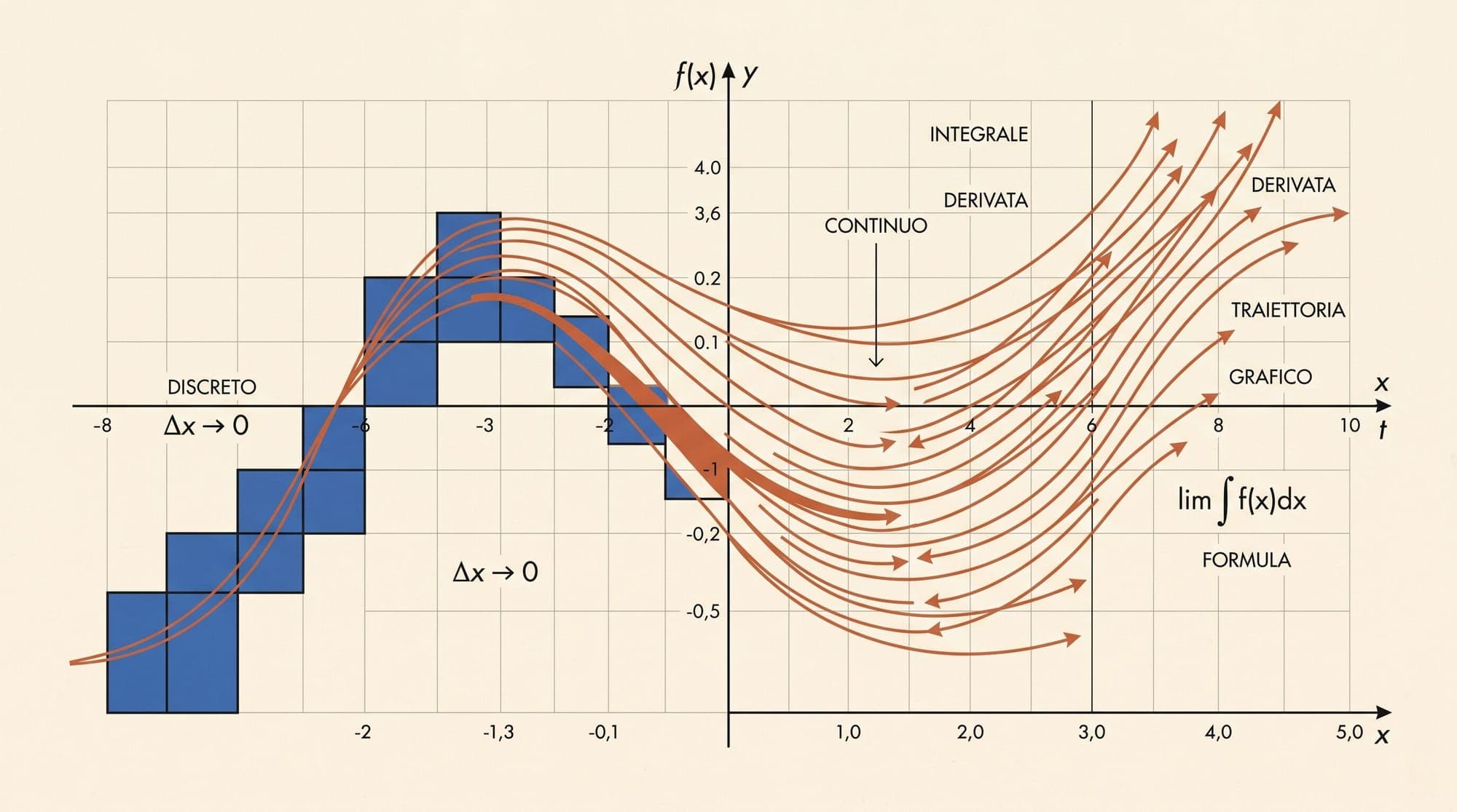
In 2018, researchers formalized a foundational insight: this discrete residual equation is an explicit Euler discretization step of a continuous ordinary differential equation (ODE). By taking the limit as layer step sizes approach zero, the hidden state transitions from a sequence of discrete activations into a continuous vector field parameterized by a neural network.

Published in Neural Ordinary Differential Equations (Chen et al., 2018), this paradigm replaced discrete feedforward computation with numerical integration. It introduced the adjoint sensitivity method to train deep continuous-depth models with constant O(1) memory overhead, fundamentally altering how machine learning frames depth, parameterization, and reversible generative modeling.

From Discrete ResNets to Continuous Vector Fields

In a conventional residual block, the activation transformation across discrete layer index t can be rewritten by introducing a step size \Delta t:

h_{t+1} = h_t + \Delta t \cdot f(h_t, \theta_t)

Rearranging the terms yields a finite difference quotient:

(h_{t+1} - h_t) / \Delta t = f(h_t, \theta_t)

Taking the continuous limit as \Delta t \to 0 transforms the discrete recurrence into a continuous differential equation:

\frac{d\mathbf{z}(t)}{dt} = f(\mathbf{z}(t), t, \theta)

Here, \mathbf{z}(t) represents the continuous hidden state trajectory over a continuous integration interval [t_0, t_1], while f(\mathbf{z}(t), t, \theta) is a neural network (such as a multi-layer perceptron or convolutional network) parameterizing the instantaneous velocity vector field.

Discrete ResNet:
Input z(0) ──>[ Layer 1 ]──> z(1) ──>[ Layer 2 ]──> z(2) ──>[ Layer 3 ]──> Output z(3)
                    (Fixed discrete evaluation steps)

Neural ODE:
Input z(t_0) ───[ Continuous ODE Solver: dz/dt = f(z(t), t, \theta) ]───> Output z(t_1)
                 (Adaptive step size along continuous time continuum)

Instead of running a fixed number of neural layers, computing the network output corresponds to solving an initial value problem (IVP):

\mathbf{z}(t_1) = \mathbf{z}(t_0) + \int_{t_0}^{t_1} f(\mathbf{z}(t), t, \theta) \, dt

The output hidden state \mathbf{z}(t_1) is evaluated using established black-box numerical ODE solvers, such as fourth-order Runge-Kutta (RK4) or adaptive step-size solvers like Dormand-Prince (dopri5).

Adaptive Solvers and the Compute-Precision Trade-off

In discrete neural networks, inference compute is fixed by architectural depth. A 50-layer network executes exactly 50 forward passes regardless of input difficulty.

Neural ODEs decouple the model specification from the numerical evaluation budget. Adaptive ODE solvers monitor local truncation error across steps:

1. Error Estimation: The solver calculates higher-order and lower-order approximations (for example, 5th-order and 4th-order in dopri5) at candidate step \Delta t.
2. Tolerance Comparison: It assesses whether the discrepancy between approximations satisfies user-defined relative (rtol) and absolute (atol) error tolerances.
3. Step Size Adaptation: If the error exceeds the tolerance, the step is rejected and recomputed with a smaller step size. If the error is well below tolerance, the step size increases for subsequent intervals.

This decoupling gives continuous-depth architectures unique operational properties:

• Tunable Inference Latency: Lowering error tolerances during deployment reduces the Number of Function Evaluations (NFE), enabling faster inference at the cost of slight numerical drift.
• Input-Dependent Compute: Simple inputs flow through smooth vector fields requiring few solver steps, while complex inputs automatically trigger finer discretization steps without architectural modifications.

The Adjoint Sensitivity Method: Constant O(1) Memory Backpropagation

The primary obstacle in training continuous differential equations with standard automatic differentiation is memory consumption. Backpropagating through a numerical solver requires caching every intermediate evaluation step, resulting in memory usage proportional to the total number of solver steps.

To eliminate this memory bottleneck, Chen et al. (2018) adapted Pontryagin's Adjoint Sensitivity Method (Pontryagin et al., 1962) for continuous backpropagation.

The Adjoint State Dynamics

Let L(\mathbf{z}(t_1)) be a scalar loss function evaluated on the output state. The adjoint state \mathbf{a}(t) is defined as the gradient of the loss with respect to the continuous hidden state at time t:

\mathbf{a}(t) = \frac{\partial L}{\partial \mathbf{z}(t)}

By applying the continuous chain rule over an infinitesimal time step, the adjoint state evolves backward in time according to its own ordinary differential equation:

\frac{d\mathbf{a}(t)}{dt} = - \mathbf{a}(t)^T \frac{\partial f(\mathbf{z}(t), t, \theta)}{\partial \mathbf{z}(t)}

To compute parameter gradients \frac{\partial L}{\partial \theta}, the system integrates the vector-Jacobian product over the full time interval:

\frac{\partial L}{\partial \theta} = - \int_{t_1}^{t_0} \mathbf{a}(t)^T \frac{\partial f(\mathbf{z}(t), t, \theta)}{\partial \theta} \, dt

The Reverse Integration Process

During standard backpropagation in discrete networks, intermediate activations must be held in VRAM throughout the forward pass. In contrast, the adjoint method computes gradients by solving an augmented ODE backward from t_1 to t_0:

Forward Pass:
z(t_0) ─────────────────[ Integrate forward: dz/dt = f ]─────────────────> z(t_1) -> Loss L
(No activation checkpoints saved to VRAM)

Backward Pass:
a(t_0), dL/d\theta <───[ Integrate backward: d[z, a, dL/d\theta]/dt ]<─── a(t_1) = dL/dz(t_1)
(Reconstructs z(t) and calculates gradients simultaneously in reverse)

The augmented state combines the hidden state, the adjoint vector, and the parameter gradient accumulator:

\mathbf{s}(t) = \begin{bmatrix} \mathbf{z}(t) \\ \mathbf{a}(t) \\ \frac{\partial L}{\partial \theta} \end{bmatrix}, \quad \frac{d\mathbf{s}(t)}{dt} = \begin{bmatrix} f(\mathbf{z}(t), t, \theta) \\ -\mathbf{a}(t)^T \frac{\partial f(\mathbf{z}(t), t, \theta)}{\partial \mathbf{z}(t)} \\ -\mathbf{a}(t)^T \frac{\partial f(\mathbf{z}(t), t, \theta)}{\partial \theta} \end{bmatrix}

Because the forward state \mathbf{z}(t) is reconstructed on the fly by reverse integration, the memory footprint during training remains constant O(1) with respect to network depth and solver steps.

Continuous Normalizing Flows and Exact Likelihood Estimation

Beyond standard supervised learning, Neural ODEs established the foundation for continuous-time generative models through Continuous Normalizing Flows (CNFs).

In discrete normalizing flows (such as RealNVP or Glow), data points are mapped to a simple base distribution (like a standard Gaussian) through a composition of invertible bijective transformations. Computing exact log-likelihoods requires evaluating the determinant of the Jacobian matrix:

\log p_X(x) = \log p_Z(z) - \sum_{k=1}^K \log \left| \det \left( \frac{\partial f_k}{\partial z_{k-1}} \right) \right|

Constraining discrete layers to have tractable triangular Jacobians severely limits model expressiveness and requires specialized bipartite coupling architectures.

The Instantaneous Change of Variables

In a continuous vector field \frac{d\mathbf{z}(t)}{dt} = f(\mathbf{z}(t), t, \theta), probability density evolution is governed by the continuous continuity equation. The change in log-probability over time simplifies to the matrix trace of the Jacobian rather than a full determinant:

\frac{\partial \log p(\mathbf{z}(t))}{\partial t} = - \text{Tr}\left( \frac{\partial f(\mathbf{z}(t), t, \theta)}{\partial \mathbf{z}(t)} \right)

Integrating this scalar differential equation along the ODE trajectory yields the exact log-likelihood of any data point x = \mathbf{z}(t_1):

\log p(\mathbf{z}(t_1)) = \log p(\mathbf{z}(t_0)) - \int_{t_0}^{t_1} \text{Tr}\left( \frac{\partial f(\mathbf{z}(t), t, \theta)}{\partial \mathbf{z}(t)} \right) \, dt

Free-Form Dynamics with FFJORD

While computing the exact trace of an N \times N Jacobian matrix scales as O(N^2) or requires N backward evaluations, Grathwohl et al. (2018) introduced FFJORD (Free-form Continuous Dynamics for Scalable Reversible Generative Models). FFJORD applies Hutchinson's trace estimator:

\text{Tr}(J) = \mathbb{E}_{p(\epsilon)} \left[ \epsilon^T J \epsilon \right]

By sampling random noise vectors \epsilon \sim \mathcal{N}(0, I) (or Rademacher distributions), the trace is estimated unbiasedly using a single vector-Jacobian product \epsilon^T J, enabling unconstrained, arbitrary neural network architectures in generative flows with O(N) compute.

Topological Limitations and Augmented Neural ODEs

Despite their theoretical appeal, vanilla Neural ODEs possess an intrinsic geometric constraint: the Picard-Lindelöf theorem guarantees that trajectories in autonomous, Lipschitz-continuous vector fields cannot intersect.

As established by Dupont et al. (2019), this continuous uniqueness property means Neural ODEs represent homeomorphic transformations that preserve topology. Consequently, standard Neural ODEs cannot:

1. Change Connected Components: Map a single connected region into disconnected decision regions.
2. Untangle Nested Geometries: Disentangle concentric circular datasets (such as an inner disc belonging to Class A surrounded by an outer ring belonging to Class B) in two dimensions without tearing space.

Topological Bottleneck in 2D Space:
Outer Ring (Class B) ───[ Non-crossing continuous trajectories ]───> Cannot cross inner disc
Inner Disc (Class A) ───[ Trajectories cannot intersect in 2D  ]───> Severe vector field stiffness

Augmented Neural ODE Solution:
Input [x_1, x_2] ───[ Pad with extra dimensions: [x_1, x_2, 0, 0] ]───> Lifted Space
Trajectories cross above and below each other without intersecting in higher dimensions.

To solve this limitation, Dupont et al. (2019) introduced Augmented Neural ODEs (ANODEs). By augmenting the input space with additional zero-initialized dimensions \mathbf{z}(t) = [\mathbf{x}(t), \mathbf{0}]^T, trajectories gain extra degrees of freedom to route around each other in higher-dimensional space without intersecting. This structural augmentation eliminates vector field stiffness, reduces NFE counts, and accelerates both training and inference.

Technical Trade-offs and the Modern Generative Lineage

While continuous-depth modeling provides theoretical clarity, its deployment involves specific engineering trade-offs:

• Computational Cost during Training: Although the adjoint method guarantees constant memory O(1), adaptive solvers may require hundreds of function evaluations per step if the learned vector field becomes stiff or chaotic, slowing wall-clock training times compared to discrete layers.
• Numerical Drift in Reverse Reconstruction: Integrating backwards from t_1 to t_0 to reconstruct \mathbf{z}(t) can accumulate numerical errors in stiff systems. Practical implementations often store sparse trajectory checkpoints to stabilize reverse solves.
• Continuous Time-Series Modeling: Neural ODEs excel in modeling irregularly sampled physical measurements (medical telemetry, climate sensors), where inputs arrive at arbitrary time intervals t_i rather than uniform discrete ticks.

The conceptual framework of continuous vector fields directly catalyzed modern generative AI architectures. The continuous formulation of score-based diffusion models (Song et al., 2020) and contemporary Flow Matching (Lipman et al., 2022) build directly on the differential equation foundations established by Neural ODEs, replacing complex diffusion stochastic differential equations with straight-path probability velocity fields.

Sources

• Neural Ordinary Differential Equations (Chen et al., 2018)
• Augmented Neural ODEs (Dupont, Doucet, & Teh, 2019)
• FFJORD: Free-form Continuous Dynamics for Scalable Reversible Generative Models (Grathwohl et al., 2018)
• Flow Matching for Generative Modeling (Lipman et al., 2022)
• Score-Based Generative Modeling through Stochastic Differential Equations (Song et al., 2020)
• A Proposal on Machine Learning via Dynamical Systems (Weinan E, 2017)