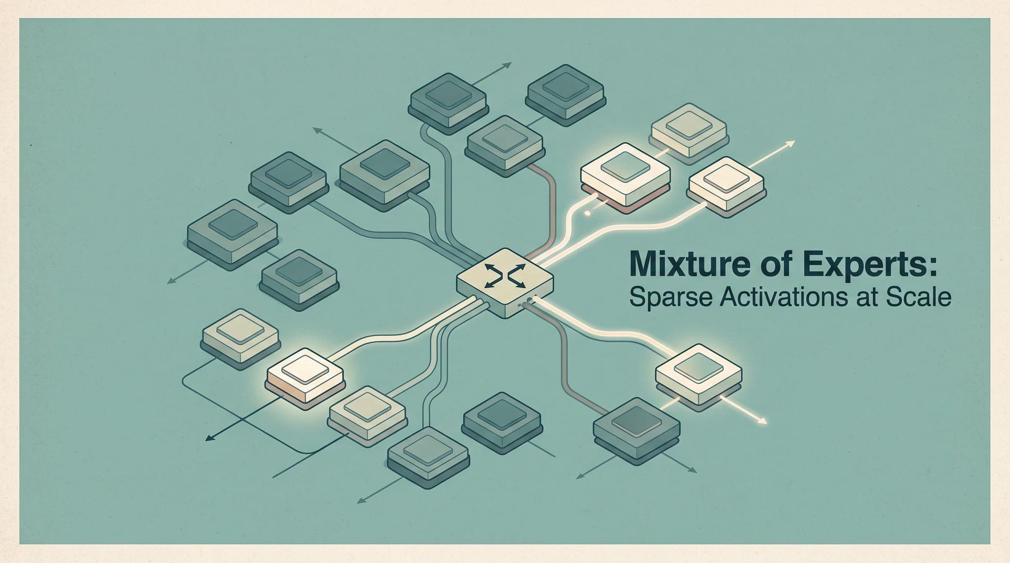
Mixture of Experts: How Sparse Activations Scale Models to Trillions of Parameters Without Trillion-Dollar Bills

In a dense transformer, every parameter participates in every forward pass. The feed-forward layer — a two-layer perceptron with a hidden expansion of four to eight times the model dimension — alone accounts for roughly two thirds of the FLOPs per token. Scale the model, and cost scales linearly: 10 times the parameters means roughly 10 times the compute at inference, 10 times the memory bandwidth, 10 times the money.

Mixture of Experts (MoE) attacks that tradeoff directly. Instead of one large feed-forward block per layer, an MoE layer holds a pool of smaller expert networks — typically dozens or hundreds. A lightweight router evaluates each incoming token and selects the top-k experts (usually k=1 or k=2) to run on it. The rest stay idle. The model can contain 400 billion or 600 billion parameters, but only the parameters in the top-k experts — a fraction of the total — consume compute for any given token.

The payoff is concrete. DeepSeek-V3 reaches 671 billion total parameters while activating only 37 billion per token, achieving GPT-4-level performance at a fraction of the compute cost of a dense model of comparable quality. Mixtral 8x7B carries 46 billion parameters but costs the same compute at inference as a 12 billion-parameter dense model, because only 12 billion parameters run per forward pass.

This is not just a research trick. MoE now powers most frontier models — DeepSeek-V3, Kimi K2, Mistral Large 3, Grok, and the majority of open-weight releases in 2025 — because it is the only practical path to scaling beyond the dense parameter ceiling without a proportional scaling in hardware cost.

The Core Architecture: Experts and Routers

An MoE layer replaces the single feed-forward network (FFN) in a standard transformer block with N parallel FFN "experts," each an independent two-layer perceptron with its own parameters. The router — itself a small learned linear projection of the token's hidden state — produces a score for every expert. Only the top-k experts by score receive the token; their outputs are weighted by the router's normalized scores and summed to produce the layer's output.

Mathematically, for an input token with hidden state x, the layer output is the weighted sum over the active expert set A (the top-k experts):

y = sum(g_i(x) * E_i(x) for i in A)

where E_i is the parameter set of expert i and g_i(x) is the router's normalized affinity for that expert. The gating function typically computes raw scores as a linear projection: H_i(x) = x . W_g + noise, then applies a softmax after masking away non-top-k experts. The Gaussian noise term (from Noisy Top-k routing) prevents the router from collapsing early in training toward a fixed subset of experts.

Dense vs. sparse activation. In a dense model, all parameters are active for every token. In MoE, only the experts selected by the router fire — the rest contribute nothing to that forward pass. The model's total parameter count can be far larger than what the activation budget allows, because only a tiny slice of parameters consumes compute at any moment.

Shared experts. Most production MoE models (DeepSeek-V3, Llama 4 Maverick) also include a small number of "shared experts" that process every token, regardless of routing. This provides a baseline capacity for handling general-purpose patterns and prevents the model from degrading on common tokens that no specialized expert claims.

Routing Strategies: Which Expert for Which Token?

Token Choice Routing

The dominant strategy in all major MoE models. Each token independently evaluates the router and selects its own top-k experts. The routing decision is local to each token — "this token goes to experts 3 and 7." This is simple and causal, which matters for autoregressive generation, but it can leave some experts overloaded while others sit idle.

Expert Choice Routing

Here the control flow inverts: each expert declares its fixed computational budget, then selects the top-N tokens it wants to process. Rather than choosing experts, tokens are claimed by experts. This guarantees full expert utilization by construction — no expert ever waits idle because it has picked exactly as many tokens as it can handle. However, expert choice creates a future-token leakage problem: an expert decides which tokens to process after seeing all tokens in the sequence, which violates the causal structure needed for left-to-right text generation. This makes expert choice attractive for bidirectional encoders but problematic for autoregressive decoders.

No-Auxiliary-Loss Load Balancing

DeepSeek-V3 introduced a routing bias that is updated outside of backpropagation. Each expert gets a scalar bias term added to its routing score. After each training step, the bias for overloaded experts is increased (making them less likely to be selected) and the bias for underloaded experts is decreased (making them more attractive). This happens on a fixed update schedule — not through gradients — which removes the tension between the load-balancing objective and the task objective. The paper reports that this eliminates expert collapse without the hyperparameter tuning that auxiliary losses require, though it does note that a very small complementary sequence-level balance loss is still used.

The Capacity Factor

The capacity factor is a hard constraint on how many tokens any single expert can handle. A capacity factor of 1.25 means each expert can accept 25% more tokens than a perfectly uniform distribution would give it. Tokens that exceed the capacity are either dropped (dropping MoE) or handled with dynamic scheduling (dropless MoE). Models like GPT-OSS, Llama 4, and DBRX use dropless MoE to avoid accuracy loss, while DeepSeek-V3 uses a 1.25 capacity factor with token dropping. The capacity factor sets an upper bound on load imbalance, which reduces how hard the auxiliary loss has to work to maintain balance.

Expert Parallelism: Distributing Experts Across Hardware

The memory footprint of an MoE model scales with the total parameter count, not the number of active parameters. A 671 billion-parameter MoE model like DeepSeek-V3 cannot fit on a single GPU even though only 37 billion parameters activate per token. Expert Parallelism (EP) distributes different experts across different GPUs, so each device holds only a subset of the full expert pool in memory. This contrasts with Tensor Parallelism, which splits individual matrix operations within a single expert across multiple GPUs.

The communication pattern differs: tensor parallelism communicates at every layer to stitch together partial matrix results; expert parallelism communicates primarily during routing — tokens for remote experts are sent across devices during the forward pass. This maps cleanly to MoE's sparse activation pattern: only routed tokens trigger inter-device traffic.

At large scale — distributing experts across 8 or more GPUs — a technique NVIDIA calls Wide Expert Parallelism reduces weight-loading pressure per device and improves arithmetic intensity in batched expert matrix multiplication. On GB200 NVL72 systems, Wide-EP achieves up to 1.8x higher per-GPU throughput compared to smaller EP configurations. DeepSeek-V3 on 256 H100s reaches 250 TFLOPs/sec/GPU, approaching theoretical hardware limits.

Serving Economics: Performance vs. Cost in Production

MoE models are memory-bound, not compute-bound, at serving time. The paradox is that they use fewer FLOPs per token than dense models of comparable quality, but require more memory: every expert must reside in addressable memory to enable dynamic routing decisions, even though most experts stay idle for any given token.

DeepSeek-R1 at full activation requires 13,719 GB/s of memory bandwidth — achievable only on data center systems consuming over 10,000 watts. At batch size 1, the bandwidth drops to 1,040 GB/s, manageable on consumer-grade GPUs. Production serving at scale cannot rely on such constrained conditions.

Inference frameworks now include MoE-specific optimizations. vLLM's V1 release integrates FlashInfer with autotuning for MoE kernels, benchmarking different configurations at startup and selecting the best. TensorRT-LLM provides custom attention kernels, inflight batching, quantization down to FP4 and INT4, and reaches over 10,000 output tokens per second at peak throughput for 64 concurrent requests. Optimized production deployments achieve 300 to 600 tokens per second per user using continuous batching, paged KV cache, and FlashAttention-3.

The tradeoff is explicit. An MoE model delivers a larger effective model for the same per-token compute cost — but at the cost of higher memory bandwidth requirements and more complex serving infrastructure. Whether that tradeoff pays off depends on the workload: for high-throughput, low-latency production serving, the memory ceiling and routing overhead can erode the compute savings. For workloads where parameter count matters more than latency, MoE makes trillion-parameter models economically viable where they would otherwise be unreachable.

Deployment Constraints and Trade-offs

Beyond the architecture itself, several hard constraints shape when and how MoE is practical:

Token dropping. When an expert's capacity is exceeded, excess tokens are dropped. This introduces accuracy loss — those tokens pass through the layer essentially unprocessed. Dropless MoE strategies (GPT-OSS, Llama 4) avoid this through dynamic scheduling but add complexity.

Routing overhead. The router itself consumes compute. For models with many experts, the routing decision can become a bottleneck, especially at small batch sizes.

Reproducibility. Because routing decisions are stochastic and data-dependent, MoE models produce different internal activation paths for identical inputs under different batch compositions. This complicates caching, debugging, and reproducibility guarantees.

Load imbalance. Even with auxiliary losses, expert utilization varies by workload. A model that routes evenly on benchmark data may collapse on production traffic that favors a narrow token distribution.

KV cache cost. All MoE experts share the same KV cache, which scales with total model depth rather than expert count. But MoE models tend to be deep and have large hidden dimensions, so the KV cache footprint remains significant despite sparse activation.

Sources

• Mixture of Experts in Large Language Models, Zhang et al., 2025 — comprehensive survey covering Noisy Top-k routing, load balancing objectives, expert choice vs. token choice, and theoretical capacity.
• A Visual Guide to Mixture of Experts (MoE) in LLMs, Maarten Grootendorst, 2024 — visual walkthrough of experts, routers, and the dense-vs-sparse distinction.
• Mixture-of-Experts (MoE) LLMs, Cameron R. Wolfe, 2024 — analysis of capacity factors, auxiliary losses, and DeepSeek-V3's bias-based load balancing.
• Expert Parallelism in TensorRT-LLM, NVIDIA — tensor vs. expert parallelism, hybrid EP/TP, and the moe_tp_size/moe_ep_size flags.
• Scaling Large MoE Models with Wide Expert Parallelism on NVL72, NVIDIA, 2025 — Wide-EP, GroupGEMM optimization, and per-GPU throughput gains.
• Deep dive: MoE inference support for Neuron, AWS — MoE layer anatomy, router APIs, and dropless vs. dropping strategies.
• Load Balancing Strategy in MoE LLMs, Hugging Face, 2025 — evolution from auxiliary losses to DeepSeek-V3's loss-free bias method.
• Auxiliary-Loss-Free Load Balancing for MoE, 2024 — the bias-based load balancing algorithm and future-token leakage analysis in expert choice.
• Mixture of Experts Infrastructure, Introl, 2025 — serving economics, memory bandwidth requirements, and production throughput numbers.
• Mixture of Experts, CMU 15-780, Aditi Raghunathan — mathematical formulation of routing, capacity factors, and load balancing.
• DeepSeek-V3 paper, 2024 — 671B total parameters, 37B active, 256 experts with 8 active per token.