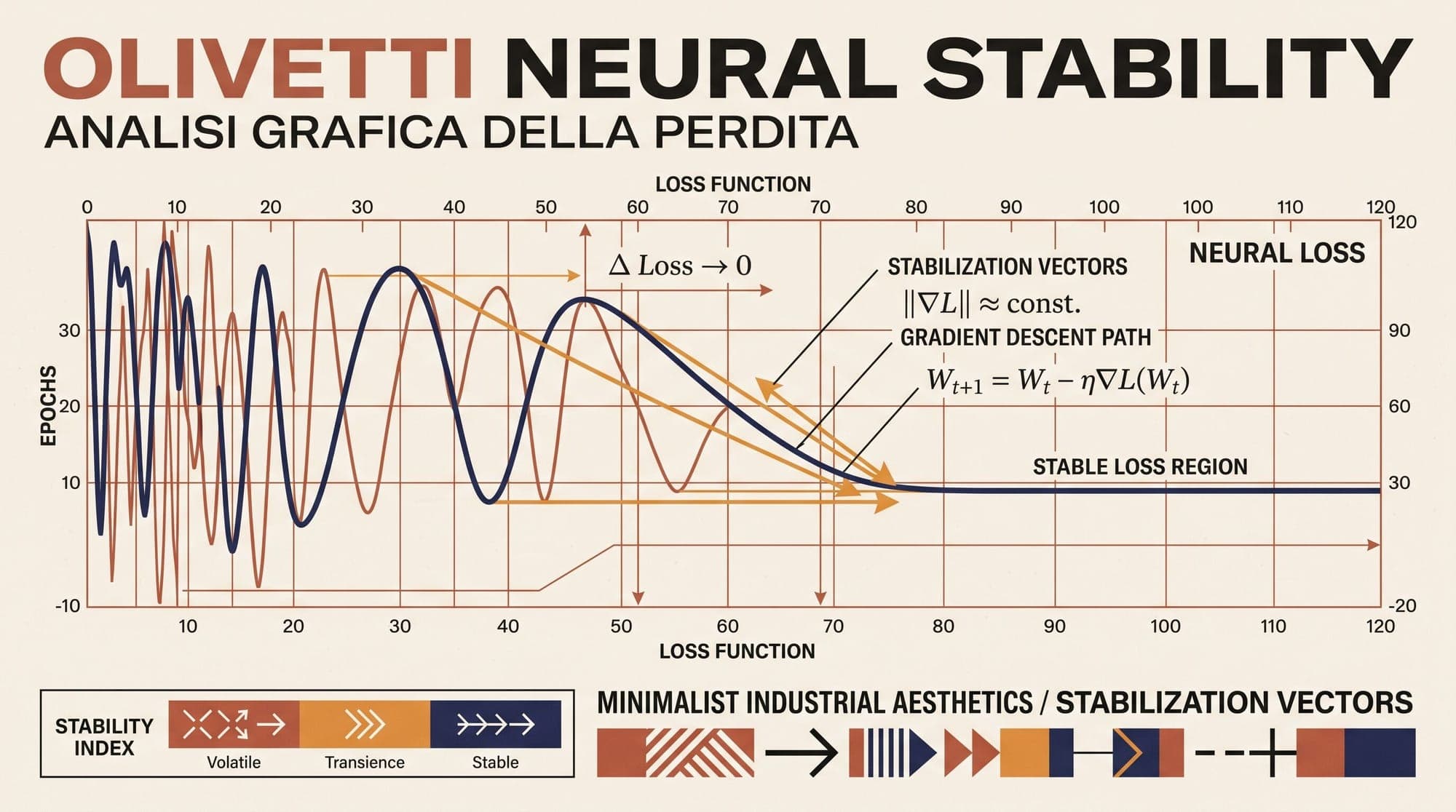
Loss Spikes and Training Stability in Large Language Models: How Attention Logit Drift, z-loss, and QK-Norm Prevent Gradient Explosions

During the pre-training of modern large language models, few operational failures are as costly as loss spikes. When training clusters containing thousands of GPUs run for weeks across trillions of tokens, a sudden, discontinuous surge in cross-entropy loss can corrupt optimizer momentum buffers, induce numerical overflow in half-precision representations, and permanently degrade downstream model capabilities. In severe cases, models experience catastrophic divergence, forcing engineering teams to roll back checkpoints, alter data ordering, or discard days of compute.

Historically, frontier engineering teams treated loss spikes as transient anomalies to be mitigated with manual heuristics: rolling back model weights by 100 to 200 steps, skipping the offending batch of training tokens, and resuming with modified learning rates. However, empirical investigations across architectures such as OPT, PaLM, GLM, Gemma, and Chameleon have revealed that loss spikes are deterministic consequences of specific mathematical and architectural vulnerabilities in deep Transformers.

Understanding the root mechanisms behind training instability (including attention logit explosion, vocabulary logit drift, embedding gradient shocks, and loss landscape geometry) has enabled the development of principled architectural safeguards: z-loss regularization, QK-normalization, attention logit soft-capping, and refined normalization schedules.

Anatomy of a Loss Spike

A loss spike is characterized by a rapid, non-linear increase in the training loss over a small number of optimization steps, typically accompanied by an explosive increase in the global gradient norm:

$\|g\|_2 = \sqrt{\sum_{i} \|\nabla_{\theta_i} \mathcal{L}\|_2^2}$

In adaptive optimizers such as AdamW, the update rule depends on the exponentially decaying moving averages of past gradients ( $m_t$ ) and squared gradients ( $v_t$ ):

$m_t = \beta_1 m_{t-1} + (1 - \beta_1) g_t$

$v_t = \beta_2 v_{t-1} + (1 - \beta_2) g_t^2$

$\theta_{t+1} = \theta_t - \frac{\eta}{\sqrt{\hat{v}_t} + \epsilon} \hat{m}_t - \eta \lambda \theta_t$

When an extreme gradient $g_t$ enters these buffers, the first moment $m_t$ absorbs a massive shock that persists across hundreds of subsequent optimization steps, even if subsequent batch gradients return to normal levels. Furthermore, the second moment $v_t$ scales up, causing the effective step size for those parameters to contract unpredictably before decaying back to baseline.

Training Step ->
Loss Trajectory:
 2.80 |----------------------\
 2.60 |                       \
 2.40 |                        \___________
 2.20 |                                    \
 2.00 |_________/\/\________________________\__/\_ (Normal decay)
       -------------------------------------------
       Step 42,100: Normal loss ~ 1.95, ||g||_2 ~ 0.8
       Step 42,105: Anomaly occurs, ||g||_2 jumps to 48.5
       Step 42,108: Loss spikes to 2.85 (Catastrophic spike)
       Step 42,200: Loss recovers to 2.15 (Permanent perplexity degradation)

Loss spikes fall into two primary categories:

Recoverable Transient Spikes: The loss jumps sharply but gradually recovers toward the baseline trajectory over dozens or hundreds of steps. While training continues, the post-recovery loss curve often settles at a slightly worse perplexity asymptote than an uncorrupted run.
Unrecoverable Divergent Spikes: The loss jumps toward near-random initialization values (e.g., $\mathcal{L} \approx \ln(|\mathcal{V}|)$ ), output activations produce NaN or Inf values under 16-bit precision, and gradient norms reach machine limits, destroying model weights irrecoverably.

Mathematical and Structural Root Causes

Loss spikes do not occur at random. They stem from interactions between multi-head self-attention mechanics, loss landscape geometry, vocabulary projection layers, and low-precision floating-point formats.

1. Attention Logit Growth and Entropy Collapse

In standard scaled dot-product attention, queries $Q \in \mathbb{R}^{N \times d_k}$ and keys $K \in \mathbb{R}^{N \times d_k}$ are projected from token representations $X$ :

$S_{ij} = \frac{q_i^T k_j}{\sqrt{d_k}}$

$A_{ij} = \text{softmax}(S_{i,:})_j = \frac{\exp(S_{ij})}{\sum_{m} \exp(S_{im})}$

During training, as parameter norms $\|W_Q\|_F$ and $\|W_K\|_F$ grow, the dot products $q_i^T k_j$ can grow arbitrarily large. Although the $\frac{1}{\sqrt{d_k}}$ scaling factor controls variance under unit-variance initialization, it does not constrain unbounded growth during hundreds of thousands of optimizer updates.

When maximum attention logits exceed values such as 50 or 100:

The softmax function saturates, collapsing into a sharp, near-one-hot probability distribution where one token receives $A_{ij} \approx 1.0$ and all other tokens receive $A_{im} \approx 0$ .
The entropy of the attention distribution $H(A_i) = -\sum_j A_{ij} \ln A_{ij}$ collapses to zero.
The derivative of softmax with respect to its input approaches zero for saturated tokens ( $\frac{\partial A_{ij}}{\partial S_{im}} = A_{ij}(\delta_{jm} - A_{im}) \to 0$ ), causing gradient vanishing across most contextual paths, while the attended token experiences sharp gradient spikes that propagate backward into query and key projection matrices.

2. Output Vocabulary Logit Drift and the Softmax Partition Function

At the final layer of a language model, hidden states $h_N \in \mathbb{R}^{d_{\text{model}}}$ are projected to vocabulary logits $z \in \mathbb{R}^{|\mathcal{V}|}$ via the unembedding matrix $W_U$ :

$z = h_N W_U$

The cross-entropy loss for target token $y$ is defined as:

$\mathcal{L}_{\text{CE}} = -\ln \frac{\exp(z_y)}{\sum_{k=1}^{|\mathcal{V}|} \exp(z_k)} = -z_y + \ln \sum_{k=1}^{|\mathcal{V}|} \exp(z_k) = -z_y + \ln Z$

Where $Z = \sum_{k=1}^{|\mathcal{V}|} \exp(z_k)$ is the partition function.

Because cross-entropy is shift-invariant (adding a constant $c$ to all logits leaves $\text{softmax}(z)$ unchanged), the optimization objective does not penalize the absolute magnitude of logits $z$ . Consequently, during long training runs, average logit values can drift toward large positive or negative magnitudes (e.g., $+80$ or $-120$ ).

When logits drift excessively:

In FP16 format (maximum representable value $\approx 65,504$ ), $\exp(z_k)$ overflows for $z_k > 11.09$ unless strict subtractive normalization ( $\max(z)$ subtraction) is executed.
Even with log-sum-exp stabilization, intermediate activations in backward passes and gradient computation buffers suffer severe numerical precision loss, causing sudden gradient spikes.

3. The Slingshot Effect and the Edge of Stability

Optimization dynamics research (Cohen et al., 2021) demonstrated that gradient descent with adaptive optimizers operates at the "Edge of Stability."

Let $H = \nabla^2 \mathcal{L}(\theta)$ represent the Hessian matrix of the loss function, and $\lambda_{\max}(H)$ denote its maximum eigenvalue (the maximum spectral curvature). In standard convex optimization, stability requires:

$\eta < \frac{2}{\lambda_{\max}(H)}$

In deep neural networks trained with AdamW, the model parameters often traverse narrow, highly curved ravines. When the effective step size approaches or exceeds the curvature boundary ( $\eta \lambda_{\max}(H) \ge 2$ ), the optimizer oscillates violently across the ravine walls. This "slingshot mechanism" propels the parameter trajectory out of the narrow valley into a high-loss region, generating an instantaneous loss spike before the optimizer can re-establish curvature equilibrium.

4. Embedding Gradient Shocks

In standard Transformer tokenizers with vocabularies ranging from 32,000 to 256,000 tokens, token frequency follows a power-law distribution. Rare tokens (e.g., specialized code syntax, multi-byte Unicode combinations, non-English scripts) appear infrequently in training batches.

When a rare token suddenly appears in a batch with a high prediction error, the gradient with respect to its specific embedding row $\nabla_{W_e[\text{token}]} \mathcal{L}$ can be several orders of magnitude larger than the average token gradient. Because embedding updates are sparse, this sudden large update creates an unnormalized perturbation that propagates through all downstream transformer blocks via residual connections.

Architectural Solutions and Stabilization Techniques

Modern foundation model architectures deploy multiple complementary techniques to bound activations, constrain logits, and stabilize gradient flow.

1. z-Loss Regularization (PaLM)

Introduced during the training of the 540-billion-parameter Pathways Language Model (PaLM, Chowdhery et al., 2022), z-loss addresses output vocabulary logit drift by adding an auxiliary loss term that directly penalizes large values of the log partition function $\ln Z$ :

$\mathcal{L}_z = \alpha \cdot (\ln Z)^2 = \alpha \cdot \left(\ln \sum_{k=1}^{|\mathcal{V}|} \exp(z_k)\right)^2$

The total training loss becomes:

$\mathcal{L}_{\text{total}} = \mathcal{L}_{\text{CE}} + \mathcal{L}_z = -z_y + \ln Z + \alpha (\ln Z)^2$

Where $\alpha$ is typically set to $10^{-4}$ ( $1\text{e-}4$ ).

Mathematical Effect of z-Loss

Taking the derivative of $\mathcal{L}_z$ with respect to logit $z_i$ :

$\frac{\partial \mathcal{L}_z}{\partial z_i} = 2 \alpha \ln Z \cdot \frac{\exp(z_i)}{Z} = 2 \alpha \ln Z \cdot P(y = i)$

When logits drift positive such that $Z \gg 1$ ( $\ln Z > 0$ ), $\frac{\partial \mathcal{L}_z}{\partial z_i}$ pushes all logits downward proportional to their softmax probability $P(y = i)$ . If logits become excessively negative such that $Z < 1$ ( $\ln Z < 0$ ), the penalty pushes logits upward. This constrains the log partition function near zero ( $\ln Z \approx 0 \implies Z \approx 1$ ), preventing logit drift without requiring artificial logit clipping.

import torch
import torch.nn as nn
import torch.nn.functional as F

class CrossEntropyWithZLoss(nn.Module):
    def __init__(self, z_loss_weight: float = 1e-4, eps: float = 1e-8):
        super().__init__()
        self.z_loss_weight = z_loss_weight
        self.eps = eps

    def forward(self, logits: torch.Tensor, targets: torch.Tensor) -> torch.Tensor:
        # logits shape: [batch_size * seq_len, vocab_size]
        # targets shape: [batch_size * seq_len]
        
        # Log-sum-exp: ln(Z)
        log_z = torch.logsumexp(logits, dim=-1)
        
        # Standard Cross-Entropy: -z_y + ln(Z)
        target_logits = logits.gather(dim=-1, index=targets.unsqueeze(-1)).squeeze(-1)
        ce_loss = log_z - target_logits
        
        # Auxiliary z-loss penalty: alpha * (ln Z)^2
        z_loss = self.z_loss_weight * (log_z ** 2)
        
        return (ce_loss + z_loss).mean()

2. QK-Normalization (Scaling ViT, Chameleon, Gemma 3)

QK-normalization (Dehghani et al., 2023) directly prevents attention logit explosion by applying Layer Normalization or RMSNorm to the query ( $Q$ ) and key ( $K$ ) tensors before calculating attention dot products.

In standard attention:

$S = \frac{X W_Q (X W_K)^T}{\sqrt{d_k}}$

In QK-normalized attention:

$Q = \text{RMSNorm}(X W_Q), \quad K = \text{RMSNorm}(X W_K)$

$S = \frac{Q K^T}{\sqrt{d_k}} \quad \text{or} \quad S = \gamma \cdot \frac{Q K^T}{\sqrt{d_k}}$

Where RMSNorm scales vectors to unit root-mean-square magnitude across the head dimension $d_k$ :

$\text{RMSNorm}(v) = \frac{v}{\sqrt{\frac{1}{d_k} \sum_{i=1}^{d_k} v_i^2 + \epsilon}} \odot g$

Mathematical Bound on Attention Scores

When queries and keys are unit-normalized (without learnable gain $g$ , or with initialized gain $g=1$ ):

$\|q_i\|_2 = \sqrt{d_k}, \quad \|k_j\|_2 = \sqrt{d_k}$

The dot product is bounded by the Cauchy-Schwarz inequality:

$|q_i^T k_j| \le \|q_i\|_2 \|k_j\|_2 = d_k$

Therefore, the scaled attention logit $S_{ij}$ is bounded:

$|S_{ij}| = \left| \frac{q_i^T k_j}{\sqrt{d_k}} \right| \le \frac{d_k}{\sqrt{d_k}} = \sqrt{d_k}$

For a standard head dimension $d_k = 128$ , the maximum possible pre-softmax logit is strictly bounded to $\sqrt{128} \approx 11.31$ , completely preventing attention logits from reaching saturation regimes ( $>50$ ).

class QKNormAttention(nn.Module):
    def __init__(self, d_model: int, num_heads: int, head_dim: int):
        super().__init__()
        self.num_heads = num_heads
        self.head_dim = head_dim
        self.scale = 1.0 / (head_dim ** 0.5)

        self.q_proj = nn.Linear(d_model, num_heads * head_dim, bias=False)
        self.k_proj = nn.Linear(d_model, num_heads * head_dim, bias=False)
        self.v_proj = nn.Linear(d_model, num_heads * head_dim, bias=False)
        self.out_proj = nn.Linear(num_heads * head_dim, d_model, bias=False)

        # Per-head RMSNorm for Q and K
        self.q_norm = nn.RMSNorm(head_dim, eps=1e-6)
        self.k_norm = nn.RMSNorm(head_dim, eps=1e-6)

    def forward(self, x: torch.Tensor, mask: torch.Tensor = None) -> torch.Tensor:
        B, N, _ = x.shape
        
        # Project and reshape: [B, num_heads, N, head_dim]
        q = self.q_proj(x).view(B, N, self.num_heads, self.head_dim).transpose(1, 2)
        k = self.k_proj(x).view(B, N, self.num_heads, self.head_dim).transpose(1, 2)
        v = self.v_proj(x).view(B, N, self.num_heads, self.head_dim).transpose(1, 2)

        # Apply QK-Norm across head_dim
        q = self.q_norm(q)
        k = self.k_norm(k)

        # Compute bounded attention
        scores = torch.matmul(q, k.transpose(-2, -1)) * self.scale
        if mask is not None:
            scores = scores.masked_fill(mask == 0, float('-inf'))
            
        attn_weights = F.softmax(scores, dim=-1)
        out = torch.matmul(attn_weights, v)
        
        out = out.transpose(1, 2).contiguous().view(B, N, -1)
        return self.out_proj(out)

QK-normalization is fully compatible with optimized attention kernels like FlashAttention-2 and FlashAttention-3 because normalization occurs before the fused kernel execution.

3. Logit Soft-Capping (Gemma 2, Grok)

Logit soft-capping (Gemma Team, 2024) restricts the range of pre-softmax attention logits and final vocabulary logits using a smooth hyperbolic tangent ( $\tanh$ ) function:

$\text{Logits}_{\text{capped}} = \text{Cap} \cdot \tanh\left(\frac{\text{Logits}}{\text{Cap}}\right)$

Where:

$\text{Cap}_{\text{attn}} = 50.0$ for attention matrix logits.
$\text{Cap}_{\text{final}} = 30.0$ for final vocabulary prediction logits.

Derivative and Clamping Behavior

As $\text{Logits} \to \infty$ , $\tanh\left(\frac{\text{Logits}}{\text{Cap}}\right) \to 1$ , ensuring $\text{Logits}_{\text{capped}} \in (-\text{Cap}, +\text{Cap})$ .

The derivative remains strictly non-zero across the entire domain:

$\frac{\partial \text{Logits}_{\text{capped}}}{\partial \text{Logits}} = 1 - \tanh^2\left(\frac{\text{Logits}}{\text{Cap}}\right)$

Unlike hard clipping ( $\text{clamp}(x, -\text{Cap}, \text{Cap})$ ), which zeros gradients when values exceed thresholds, soft-capping preserves continuous gradient backpropagation while preventing numerical overflow.

def soft_cap(logits: torch.Tensor, cap_value: float = 30.0) -> torch.Tensor:
    """Smooth hyperbolic tangent logit soft-capping."""
    return cap_value * torch.tanh(logits / cap_value)

While soft-capping provides stability during pre-training, standard implementations require customized CUDA kernels to prevent materializing un-fused intermediate tensors during self-attention computation.

Normalization Placement: Pre-LN vs. Sandwich-LN vs. DeepNorm

The placement of normalization layers governs how residual variance scales with network depth $L$ .

Post-LN (Vaswani et al., 2017):
x_{l+1} = LayerNorm(x_l + SubLayer(x_l))
-> Unstable: Gradients at output layers are magnitude O(1), but vanish at early layers O(1/sqrt(L)).

Pre-LN (Xiong et al., 2020):
x_{l+1} = x_l + SubLayer(LayerNorm(x_l))
-> Stable initialization: Gradients flow cleanly via skip connections.
-> Drawback: Residual norm grows as O(sqrt(L)), making later layers contribute proportionally less.

Sandwich-LN (CogView, GLM):
x_{l+1} = x_l + LayerNorm(SubLayer(LayerNorm(x_l)))
-> Prevents activation explosions inside sublayers.
-> Risk: Can suppress gradient backpropagation in architectures deeper than 60 layers.

DeepNorm (Wang et al., 2022):
x_{l+1} = LayerNorm(x_l * alpha + SubLayer(x_l))
Where alpha = (2L)^{1/4}, and sublayer weights are scaled by beta = (8L)^{-1/4}.
-> Retains Post-LN performance while matching Pre-LN training stability up to 1,000 layers.

Embedding Gradient Shrinking and Adaptive Clipping

To prevent rare-token embedding updates from destabilizing the residual stream, GLM (Zeng et al., 2022) introduced embedding gradient shrinking:

$g_{W_e} \leftarrow \alpha \cdot g_{W_e}$

Where $\alpha \in [0.1, 0.5]$ . This dampens updates to the embedding matrix without slowing the learning rate of internal transformer weights.

Additionally, global gradient clipping scales the collective gradient vector if its $\ell_2$ norm exceeds a threshold $M_{\text{clip}}$ (typically 1.0):

$g \leftarrow g \cdot \min\left(1, \frac{M_{\text{clip}}}{\|g\|_2}\right)$

Comparison of Stability Mechanisms

Comparing Key Stabilization Techniques

z-Loss Regularization: Applied at the output unembedding layer. Targets vocabulary logit drift and partition function overflow. Adds negligible computational overhead ( $<0.1\%$ ) and is fully compatible with FlashAttention. Adopted in PaLM, Chameleon, and DeepSeek-V3.
QK-Normalization: Applied to query and key projection vectors inside every attention head. Targets attention logit explosion and entropy collapse. Adds less than $0.5\%$ computational overhead and integrates directly with FlashAttention kernels. Adopted in ViT-22B, Gemma 3, and Chameleon.
Attention and Output Logit Soft-Capping: Applied to pre-softmax attention matrices and final vocabulary projections. Targets logit magnitude growth and output overconfidence. Requires custom fused kernels to avoid memory overhead during attention computation. Adopted in Gemma 2 and Grok-1.
Sandwich Normalization: Applied to sublayer outputs before residual additions. Targets intermediate activation blowups. Adds minimal overhead ( $<1\%$ ) but carries risks of gradient vanishing in networks exceeding 60 layers. Adopted in CogView and GLM-130B.
DeepNorm: Applied to residual stream connections via dynamic weight scaling. Targets post-LN gradient explosion. Adds zero computational overhead at runtime and is fully compatible with all attention engines. Adopted in DeepNet and GLM-4.
Embedding Gradient Shrinking: Applied to input embedding lookup tensors. Targets rare-token gradient shocks and sudden residual perturbations. Adds zero runtime overhead. Adopted in GLM and ChatGLM.

Operational Diagnostics and Anomaly Detection

In production training runs, automated telemetry systems track early indicators of instability 50 to 500 steps before a full loss spike occurs:

Attention Entropy Monitoring:

$H(A) = -\frac{1}{N} \sum_{i=1}^N \sum_{j=1}^N A_{ij} \ln A_{ij}$ A sudden drop in average attention entropy across any single head indicates logit concentration and impending saturation.

Per-Layer Gradient Norm Ratios:

Tracking $\frac{\|g_L\|_2}{\|g_1\|_2}$ highlights whether gradient energy is concentrating anomalously in the initial embeddings or final classification heads.

Maximum Logit Tracking:

Logging $\max |S_{ij}|$ across attention heads and $\max |z_k|$ on the output layer catches logit drift before it triggers half-precision exponent overflow.

By combining QK-normalization on attention heads with z-loss regularization on vocabulary projections and Pre-LN/RMSNorm residual connections, modern LLM pre-training pipelines eliminate the primary architectural drivers of loss spikes, ensuring deterministic convergence across multi-trillion token runs.