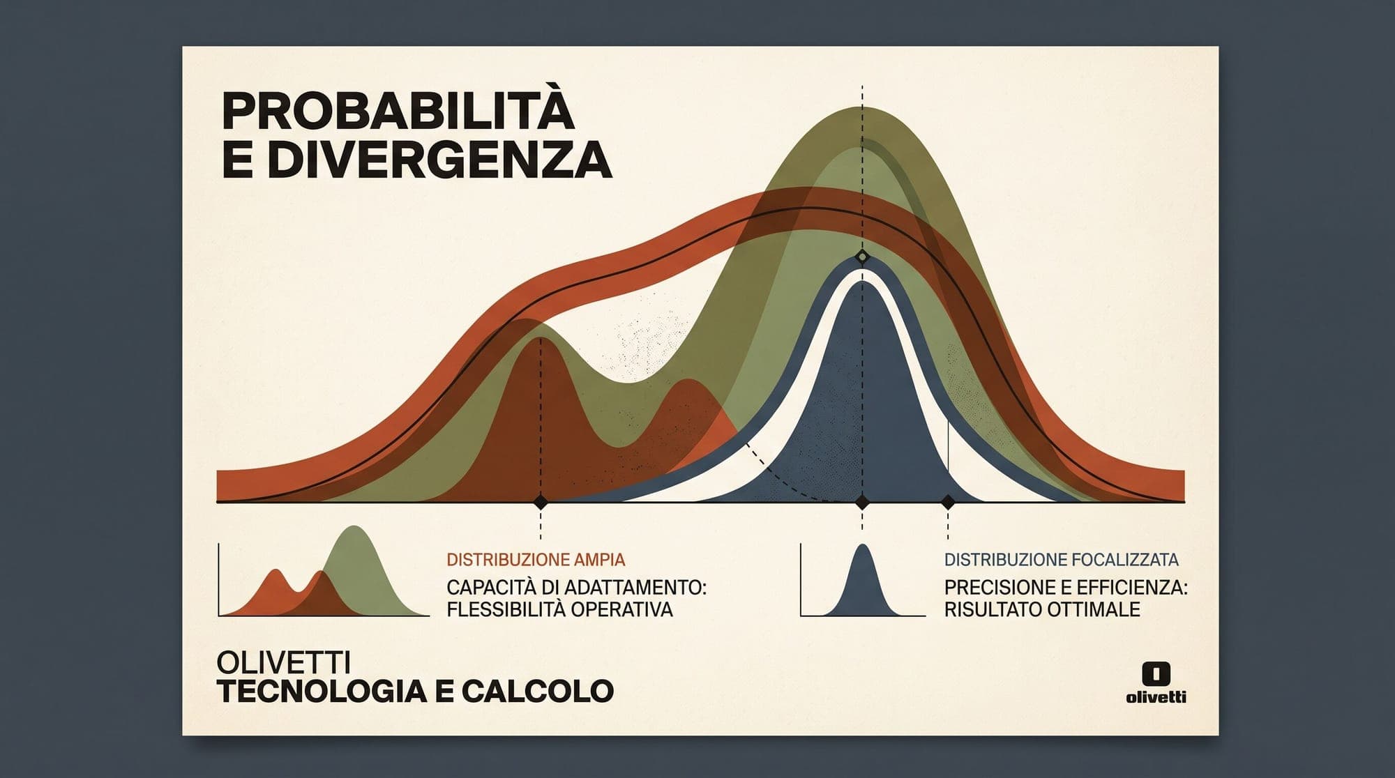
Forward KL vs. Reverse KL Divergence: Mode Covering, Mode Seeking, and the Alignment Dynamics of Large Language Models

Every phase of modern large language model development, from multi-trillion token pre-training to reinforcement learning from human feedback (RLHF) and student model distillation, fundamentally revolves around minimizing statistical distance between probability distributions. The primary mathematical tool utilized for this purpose is the Kullback-Leibler (KL) divergence, introduced by Solomon Kullback and Richard Leibler in 1951.

Despite its foundational role in objective functions across deep learning, KL divergence possesses a mathematical asymmetry: the divergence from distribution $P$ to distribution $Q$ is not equal to the divergence from $Q$ to $P$. Choosing which distribution serves as the reference and which serves as the target fundamentally changes the optimization dynamics. This mathematical distinction splits machine learning objectives into two regimes: "mode-covering" (mean-seeking) behavior via Forward KL, and "mode-seeking" (zero-forcing) behavior via Reverse KL.

Understanding this asymmetry explains why base models exhibit high output diversity but occasionally hallucinate, why RLHF alignment causes output entropy collapse, and why modern on-policy distillation enables small reasoning models to replicate the mathematical precision of frontier systems.

Mathematical Foundations: Zero-Avoiding vs. Zero-Forcing Penalties

For two continuous or discrete probability distributions $P(x)$ (the target or data distribution) and $Q(x)$ (the parameterized model distribution) defined over a common support $\mathcal{X}$, the Kullback-Leibler divergence is defined as the expected logarithmic ratio of their densities:

$$D_{\mathrm{KL}}(P \parallel Q) = \mathbb{E}_{x \sim P}\left[\log \frac{P(x)}{Q(x)}\right] = \sum_{x \in \mathcal{X}} P(x) \log \left(\frac{P(x)}{Q(x)}\right)$$

Because $D_{\mathrm{KL}}(P \parallel Q) \ge 0$ (by Jensen's inequality) and equals zero if and only if $P = Q$ almost everywhere, it acts as a directed distance metric, though it violates the triangle inequality and symmetry requirements of a formal metric space.

Forward KL: The Zero-Avoiding Property

In Forward KL divergence, denoted $D_{\mathrm{KL}}(P \parallel Q)$, the expectation is evaluated with respect to the target distribution $P$:

$$D_{\mathrm{KL}}(P \parallel Q) = \sum_{x \in \mathcal{X}} P(x) \log P(x) - \sum_{x \in \mathcal{X}} P(x) \log Q(x)$$

Consider the behavior of the term $P(x) \log \frac{P(x)}{Q(x)}$:

• If $P(x) > 0$ and the model assigns near-zero probability $Q(x) \to 0$, the ratio $\frac{P(x)}{Q(x)} \to \infty$, and the loss term explodes to infinity.
• If $P(x) = 0$ and $Q(x) > 0$, the term evaluates to $0 \log 0 = 0$.

Because the model receives an infinite penalty if it assigns zero probability to any point where data exists, Forward KL is strictly zero-avoiding. The model distribution $Q$ is forced to expand its support across all regions where $P(x) > 0$. When $P$ is a complex multimodal distribution and $Q$ possesses limited expressive capacity (such as a unimodal Gaussian or a compact neural network with bounded parameters), $Q$ must stretch across all modes. This is known as mode-covering or mean-seeking optimization. To cover multiple separated peaks, $Q$ must place substantial probability mass in the low-density valleys between modes.

Reverse KL: The Zero-Forcing Property

In Reverse KL divergence, denoted $D_{\mathrm{KL}}(Q \parallel P)$, the expectation is evaluated with respect to the parameterized model $Q$:

$$D_{\mathrm{KL}}(Q \parallel P) = \mathbb{E}_{x \sim Q}\left[\log \frac{Q(x)}{P(x)}\right] = \sum_{x \in \mathcal{X}} Q(x) \log \left(\frac{Q(x)}{P(x)}\right)$$

Analyzing the boundary conditions of Reverse KL reveals inverted optimization incentives:

• If $P(x) \to 0$ and $Q(x) > 0$, the ratio $\frac{Q(x)}{P(x)} \to \infty$, and the loss diverges to infinity.
• If $P(x) > 0$ but the model sets $Q(x) = 0$, the term evaluates to $\lim_{Q \to 0} Q \log Q = 0$, incurring exactly zero penalty.

Under Reverse KL, the model is severely punished for generating tokens where the target distribution has no density, but receives no penalty for completely ignoring modes of $P$. Consequently, Reverse KL is strictly zero-forcing. The parameterized model $Q$ minimizes loss by contracting onto a single dominant mode (or a narrow subset of modes) of $P$ where it can ensure $P(x)$ is high, entirely shedding the remaining modes. This is known as mode-seeking optimization.

Pre-Training and SFT: Maximum Likelihood as Forward KL

Autoregressive language model pre-training and supervised fine-tuning (SFT) rely on Maximum Likelihood Estimation (MLE), parameterized via cross-entropy loss over a training corpus:

$$\mathcal{L}_{\mathrm{MLE}}(\theta) = -\mathbb{E}_{x \sim P_{\mathrm{data}}}[\log P_\theta(x)]$$

Mathematically, minimizing the empirical cross-entropy loss over a dataset $P_{\mathrm{data}}$ is exactly equivalent to minimizing the Forward KL divergence between the true data-generating distribution and the model $P_\theta$:

$$\arg\min_\theta D_{\mathrm{KL}}(P_{\mathrm{data}} \parallel P_\theta) = \arg\min_\theta \left( -H(P_{\mathrm{data}}) - \mathbb{E}_{x \sim P_{\mathrm{data}}}[\log P_\theta(x)] \right) = \arg\min_\theta \mathcal{L}_{\mathrm{MLE}}(\theta)$$

Since the entropy of the data distribution $H(P_{\mathrm{data}})$ is constant with respect to model parameters $\theta$, optimizing standard cross-entropy forces the language model into the zero-avoiding, mode-covering regime.

Practical Implications for Base Models

1. Broad Expressive Coverage: Base models trained with Forward KL learn to assign probability mass to a vast spectrum of linguistic styles, domain vocabularies, reasoning strategies, and human perspectives. They capture the long-tail distribution of natural language.
2. Probability Blending and Hallucinations: When an autoregressive transformer encounters a prompt with multiple valid continuations (e.g., competing historical interpretations or multiple syntactically valid coding paths), Forward KL prevents the model from choosing just one and dropping the rest. If model capacity is insufficient to cleanly partition these modes conditionally, the model spreads probability across the boundary, generating blended, grammatically fluent nonsense (hallucinations).

Post-Training Alignment: Reverse KL in RLHF and Preference Optimization

While pre-training uses Forward KL to absorb broad language distributions, reinforcement learning alignment shifts the primary objective toward Reverse KL.

In standard Reinforcement Learning from Human Feedback (RLHF) pipelines, such as Proximal Policy Optimization (PPO) and Group Relative Policy Optimization (GRPO), the optimization objective balances reward maximization against a regularization penalty that prevents policy drift away from an initial reference model $\pi_{\mathrm{ref}}$:

$$\max_\theta \mathbb{E}_{x \sim \mathcal{D}, y \sim \pi_\theta(\cdot \mid x)}\left[ R(x, y) - \beta \log \frac{\pi_\theta(y \mid x)}{\pi_{\mathrm{ref}}(y \mid x)} \right]$$

The regularization term $\mathbb{E}_{y \sim \pi_\theta}\left[\log \frac{\pi_\theta(y \mid x)}{\pi_{\mathrm{ref}}(y \mid x)}\right]$ is the Reverse KL divergence $D_{\mathrm{KL}}(\pi_\theta \parallel \pi_{\mathrm{ref}})$.

   Forward KL (MLE / SFT)                 Reverse KL (RLHF / On-Policy Distill)
   Target P is broad/multimodal           Target P has multiple peaks

          P(x) (Data)                             P(x) (Target)
       /\             /\                       /\             /\
      /  \           /  \                     /  \           /  \
     /    \         /    \                   /    \         /    \
    /      \_______/      \                 /      \_______/      \
   -------------------------               -------------------------

         Q(x) (Model)                            Q(x) (Model)
       _________________                                      /\
      /                 \                                    /  \
     /                   \                                  /    \
    /                     \                                /      \
   -------------------------               -------------------------
    Zero-avoiding: covers all               Zero-forcing: collapses to single
    modes; places mass in valleys.          peak; ignores secondary modes.

The Mechanism of the "Alignment Tax"

Because the expectation in RLHF is taken over samples $y$ drawn from the active policy $\pi_\theta$, the optimization process enforces zero-forcing behavior:

• The policy is rewarded for finding high-density, high-reward modes in the reward landscape (e.g., structured markdown, polite disclaimers, concise bulleted answers).
• The Reverse KL penalty permits $\pi_\theta$ to assign zero probability to valid, creative, or stylistically diverse completions that $\pi_{\mathrm{ref}}$ could generate, provided $\pi_\theta$ does not produce completions that $\pi_{\mathrm{ref}}$ deems impossible.

This mathematical pressure causes the well-documented "alignment tax" and output entropy collapse: aligned models exhibit sharp, reliable compliance on common benchmarks, but sacrifice vocabulary diversity, idiosyncratic phrasing, and creative non-conformity.

Knowledge Distillation: Offline Forward KL vs. On-Policy Reverse KL

The choice between Forward and Reverse KL divergence has transformed knowledge distillation for large language models.

Offline Distillation (Forward KL)

In classical sequence-level distillation (Kim & Rush, 2016), a large teacher model $P_{\mathcal{T}}$ generates a static synthetic dataset $\mathcal{D}_{\mathcal{T}}$, and a smaller student model $P_{\mathcal{S}}$ is trained using standard cross-entropy loss on those outputs:

$$\mathcal{L}_{\mathrm{offline}} = \mathbb{E}_{(x, y) \sim \mathcal{D}_{\mathcal{T}}}\left[ -\log P_{\mathcal{S}}(y \mid x) \right] \approx D_{\mathrm{KL}}(P_{\mathcal{T}} \parallel P_{\mathcal{S}})$$

Because this objective minimizes Forward KL, the compact student model is penalized whenever it fails to cover the full diversity of the teacher's vocabulary and reasoning paths. Lacking the parameter capacity to represent the teacher's high-dimensional multimodal distribution, the student stretches its probability mass across the support, assigning high probability to invalid inter-modal tokens. This causes severe hallucination rates when compact models are trained on raw teacher rollouts.

On-Policy Distillation (Reverse KL)

To resolve this bottleneck, modern frameworks such as MiniLLM (Gu et al., 2023) and Generalized Knowledge Distillation (Agarwal et al., 2024) formulate distillation through Reverse KL divergence:

$$\mathcal{L}_{\mathrm{on\text{-}policy}}(\theta) = \mathbb{E}_{x \sim \mathcal{D}}\left[ D_{\mathrm{KL}}(P_{\mathcal{S}}(\cdot \mid x) \parallel P_{\mathcal{T}}(\cdot \mid x)) \right] = \mathbb{E}_{x \sim \mathcal{D}, y \sim P_{\mathcal{S}}(\cdot \mid x)}\left[ \log \frac{P_{\mathcal{S}}(y \mid x)}{P_{\mathcal{T}}(y \mid x)} \right]$$

In this setup:

1. The student model $P_{\mathcal{S}}$ generates its own candidate response sequences on-policy ($y \sim P_{\mathcal{S}}$).
2. The teacher model $P_{\mathcal{T}}$ evaluates the log-likelihood of the student-generated tokens.
3. Gradients are computed using policy gradient estimators (or analytical token-level approximations) to penalize the student whenever it generates sequences that the teacher considers improbable.

Because Reverse KL is zero-forcing, the student is not penalized for failing to replicate the entire broad vocabulary of the teacher. Instead, it is rewarded for mastering a compact, high-precision subset of valid reasoning trajectories. This shift explains why modern distilled reasoning models (such as DeepSeek-R1-Distill variants) retain high mathematical and algorithmic problem-solving accuracy on consumer hardware despite having up to 90% fewer parameters than their base teachers.

Beyond Binary Divergences: JSD, $f$-Divergences, and Hybrid Objectives

Neither Forward nor Reverse KL represents a universally optimal objective for every stage of model development. Recent research focuses on generalized divergence families and hybrid objectives that balance coverage against precision.

+----------------------------------------------------------------------------------------------------+
|                                    DIVERGENCE COMPARISON MATRIX                                    |
+-------------------+----------------+-----------------+-----------------------+---------------------+
| Divergence Metric | Direction      | Zero Property   | Primary LLM Role      | Main Trade-Off      |
+-------------------+----------------+-----------------+-----------------------+---------------------+
| Forward KL        | KL(P || Q)     | Zero-avoiding   | Pre-training, SFT     | High diversity;     |
|                   |                | (Mode-covering) | Offline Distillation  | hallucination risk  |
+-------------------+----------------+-----------------+-----------------------+---------------------+
| Reverse KL        | KL(Q || P)     | Zero-forcing    | RLHF (PPO/GRPO),      | High precision;     |
|                   |                | (Mode-seeking)  | On-Policy Distillation| entropy collapse    |
+-------------------+----------------+-----------------+-----------------------+---------------------+
| Jensen-Shannon    | 0.5 KL(P || M) | Symmetric,      | GANs, Distributional  | Bounded gradients;  |
| (JSD)             | + 0.5 KL(Q || M)| smoothed bound  | Preference Matching   | complex estimation  |
+-------------------+----------------+-----------------+-----------------------+---------------------+
| Alpha-Divergence  | Variational    | Interpolates    | Adaptive Distillation | Requires hyperparam |
| (D_alpha)         | interpolation  | between regimes | and Alignment         | tuning per domain   |
+-------------------+----------------+-----------------+-----------------------+---------------------+

Jensen-Shannon Divergence (JSD)

The Jensen-Shannon Divergence creates a symmetric distance metric by measuring KL divergence against an average mixture distribution $M = \frac{1}{2}(P + Q)$:

$$\mathrm{JSD}(P \parallel Q) = \frac{1}{2} D_{\mathrm{KL}}(P \parallel M) + \frac{1}{2} D_{\mathrm{KL}}(Q \parallel M)$$

Because $M$ always has support wherever either $P$ or $Q$ has support, JSD is bounded between 0 and $\log 2$ (or 1 in base-2), preventing gradient explosions and offering balanced mode retention without extreme zero-forcing collapse.

Entropy-Aware Hybrid Distillation

Recent post-training pipelines combine both objectives dynamically based on local predictive uncertainty:

• High-Entropy Token Spaces: In open-ended creative contexts where the teacher distribution exhibits high conditional entropy (such as creative writing or conversational chit-chat), the training objective applies Forward KL to preserve natural phrasing diversity.
• Low-Entropy Token Spaces: In deterministic reasoning chains (such as mathematical derivations, formal logic proofs, and API syntax), the training objective switches to Reverse KL to enforce strict mode-seeking precision and eliminate hallucinated syntax.

Summary and Engineering Rules of Thumb

When architecting training loops, distillation pipelines, and alignment objectives:

1. Use Forward KL (MLE / Standard Cross-Entropy) when the goal is foundational knowledge acquisition, multi-domain fluency, and broad contextual coverage. Expect high vocabulary richness but monitor for probability spreading in capacity-constrained models.
2. Use Reverse KL (On-Policy Policy Gradients / RLHF Regularization) when the goal is task specialization, formal reasoning, code execution accuracy, and adherence to system constraints. Expect reduced output entropy and prepare mitigation strategies if generation diversity is required.
3. Avoid Pure Offline Distillation for Sub-8B Models: Forcing a compact student to cover a frontier teacher's full distribution via Forward KL induces hallucinations. Utilize on-policy generation with teacher verification to mode-seek valid reasoning chains.

Sources

• Kullback, S., & Leibler, R. A. (1951). On Information and Sufficiency. The Annals of Mathematical Statistics, 22(1), 79-86.
• Minka, T. (2005). Divergence measures and message passing. Microsoft Research Technical Report MSR-TR-2005-173.
• Kim, Y., & Rush, A. M. (2016). Sequence-Level Knowledge Distillation. arXiv:1606.07947.
• Gu, Y., Dong, L., Wei, F., & Huang, M. (2023). Knowledge Distillation of Large Language Models (MiniLLM). arXiv:2306.08543.
• Agarwal, R., Vieillard, N., Stanczyk, P., Ramos, S., Geist, M., & Bachem, O. (2024). On-Policy Distillation of Language Models: Learning from Self-Generated Data. arXiv:2402.14811.
• Schulman, J. (2020). Approximating KL Divergence. John Schulman's Blog.
• Casper, S., et al. (2023). Open Problems and Fundamental Limitations of Reinforcement Learning from Human Feedback. arXiv:2307.15217.