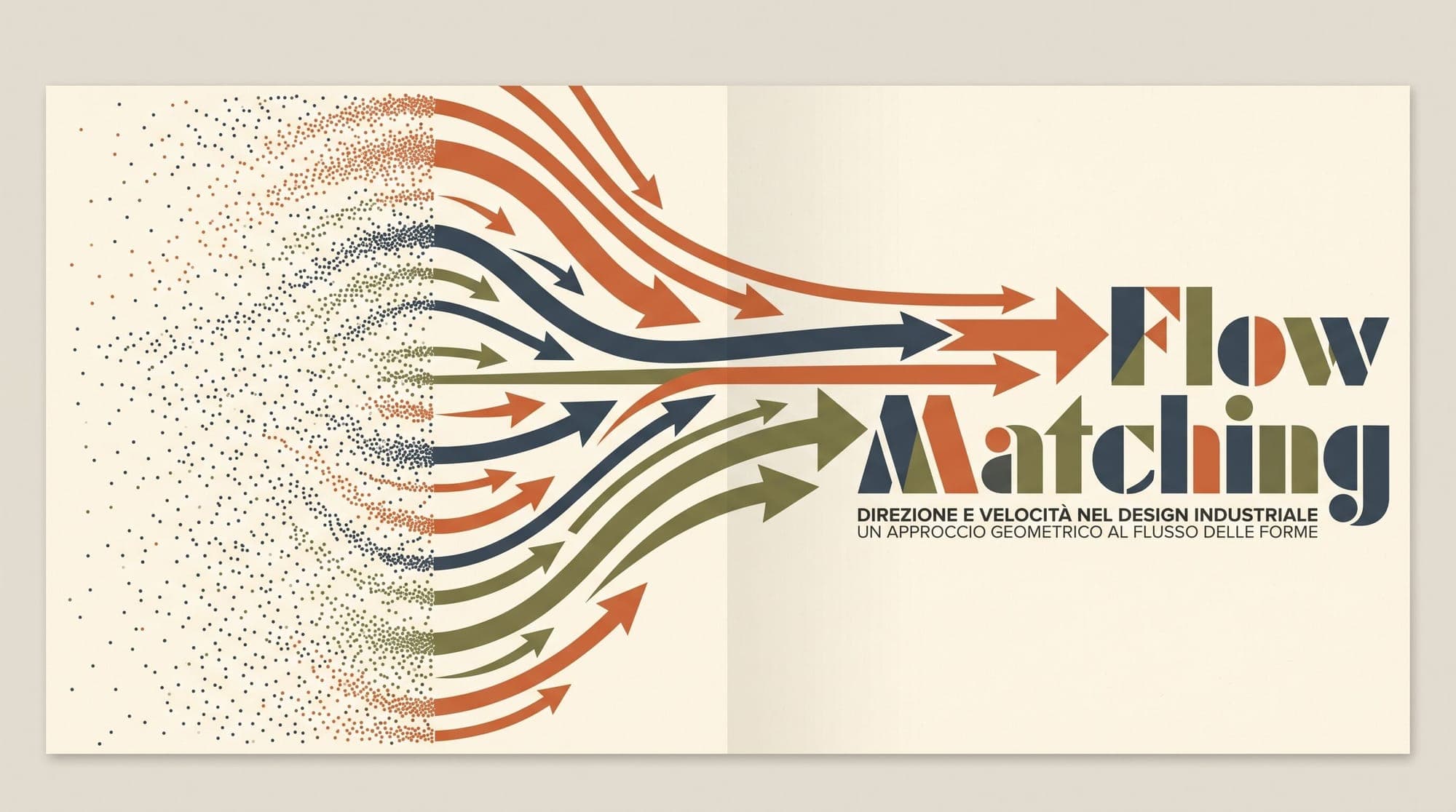
Flow Matching for Generative Modeling: How Continuous Normalizing Flows and Optimal Transport Paths Replace Diffusion SDEs

Generative modeling underwent a structural shift with the introduction of Flow Matching (FM), formulated independently by Lipman et al. (2022), Albergo and Vanden-Eijnden (2022), and Liu et al. (2022). While Denoising Diffusion Probabilistic Models (DDPM) and score-based Stochastic Differential Equations (SDEs) established state-of-the-art sample quality across vision and audio domains, their sampling dynamics rely on curved stochastic trajectories that require extensive numerical integration steps.

Continuous Normalizing Flows (CNFs) offer deterministic ordinary differential equation (ODE) sampling, exact likelihood evaluation, and clean mathematical formulation. Historically, training CNFs required integrating continuous ODE trajectories during optimization via the adjoint sensitivity method (Chen et al., 2018), making large-scale training computationally intractable. Flow Matching resolved this barrier by introducing a simulation-free, regression-based training objective that fits time-dependent vector fields along straight optimal transport paths.

Today, Flow Matching serves as the core generative backbone for frontier models including Stable Diffusion 3 (Esser et al., 2024), Flux.1, Meta Voicebox (Le et al., 2023), and MovieGen.

1. Mathematical Foundations: Continuous Normalizing Flows and Probability Paths

A Continuous Normalizing Flow defines a continuous time-dependent diffeomorphism $\phi_t: \mathbb{R}^d \to \mathbb{R}^d$ across the unit time interval $t \in [0, 1]$, governed by an ordinary differential equation:

$$\frac{d}{dt} \phi_t(x) = v_t(\phi_t(x)), \quad \phi_0(x) = x$$

where $v_t: \mathbb{R}^d \to \mathbb{R}^d$ is a time-dependent velocity vector field parameterized by a neural network with weights $\theta$.

The flow $\phi_t$ transforms a known, tractable prior distribution $p_0 = \mathcal{N}(0, I)$ at $t = 0$ into a target empirical data distribution $q(x_1) \approx p_1(x)$ at $t = 1$. The evolution of the probability density $p_t(x)$ induced by the vector field $v_t(x)$ is governed by the continuity equation, which enforces the conservation of probability mass:

$$\frac{\partial p_t(x)}{\partial t} + \nabla \cdot (p_t(x) v_t(x)) = 0$$

If one had direct access to the ground-truth marginal vector field $u_t(x)$ that generates the target probability path $p_t(x)$, training a neural network $v_t(x; \theta)$ would reduce to a simple mean-squared error regression:

$$\mathcal{L}_{FM}(\theta) = \mathbb{E}_{t \sim \mathcal{U}[0, 1], x \sim p_t(x)} \left[ \| v_t(x; \theta) - u_t(x) \|^2 \right]$$

However, calculating the marginal vector field $u_t(x)$ and sampling from the marginal path $p_t(x) = \int p_t(x|x_1) q(x_1) dx_1$ is intractable for arbitrary high-dimensional empirical data distributions $q(x_1)$.

2. The Core Breakthrough: Conditional Flow Matching (CFM)

The foundational insight of Flow Matching is that while the marginal vector field $u_t(x)$ is intractable, the conditional vector field $u_t(x|x_1)$ associated with an individual data point $x_1 \sim q(x_1)$ (or conditioned on a pair of endpoints $(x_0, x_1)$) can be constructed in closed analytical form.

Lipman et al. introduced the Conditional Flow Matching (CFM) objective:

$$\mathcal{L}_{CFM}(\theta) = \mathbb{E}_{t \sim \mathcal{U}[0, 1], x_1 \sim q(x_1), x \sim p_t(x|x_1)} \left[ \| v_t(x; \theta) - u_t(x|x_1) \|^2 \right]$$

Equivalence of Gradients Theorem

The key theoretical result established by Lipman et al. states that the gradient of the intractable marginal Flow Matching loss is strictly identical to the gradient of the tractable Conditional Flow Matching loss:

$$\nabla_\theta \mathcal{L}_{FM}(\theta) = \nabla_\theta \mathcal{L}_{CFM}(\theta)$$

Because both losses share identical gradients with respect to model parameters $\theta$, minimizing $\mathcal{L}_{CFM}(\theta)$ via stochastic gradient descent over mini-batches of training samples $x_1$ and time steps $t$ directly optimizes the true marginal vector field $v_t(x; \theta) \to u_t(x)$. Training requires no numerical ODE integration, no score estimation tricks, and no backpropagation through differential equation solvers.

3. Optimal Transport Displacement Interpolation (OT-CFM)

While arbitrary probability paths can be designed, the choice of conditional probability path $p_t(x|x_1)$ determines the geometry of the learned vector field and the resulting inference speed.

In standard Gaussian conditional paths, the distribution at time $t$ given data sample $x_1$ is parameterized as:

$$p_t(x|x_1) = \mathcal{N}(x; \mu_t(x_1), \sigma_t^2(x_1) I)$$

Under Optimal Transport Conditional Flow Matching (OT-CFM), the mean and variance schedules are defined linearly:

$$\mu_t(x_1) = t x_1, \quad \sigma_t(x_1) = 1 - (1 - \sigma_{min}) t$$

When considering paired endpoints $x_0 \sim \mathcal{N}(0, I)$ and $x_1 \sim q(x_1)$, the forward interpolation path corresponds to optimal transport displacement interpolation:

$$x_t = \psi_t(x_0, x_1) = (1 - t) x_0 + t x_1$$

The time derivative of this interpolation yields a constant, time-invariant conditional vector field:

$$u_t(x_t | x_0, x_1) = \frac{d}{dt} \psi_t(x_0, x_1) = x_1 - x_0$$

Why Straight Paths Matter

In score-based diffusion models (such as Variance Preserving SDEs), the generative process simulates time-reversed Brownian motion. The forward process injects noise at every infinitesimal step, forcing the reverse trajectories to follow curved paths through high-dimensional space. Numerical ODE/SDE solvers (such as DDIM or Euler-Maruyama) accumulate significant truncation errors when step sizes are increased, requiring 30 to 50 function evaluations (NFE) for high-fidelity generation.

In contrast, Optimal Transport Flow Matching defines straight line paths between noise $x_0$ and data $x_1$. Because the velocity vector along each trajectory $x_1 - x_0$ is constant:

• Directional derivative variations along trajectories approach zero.
• Numerical integration errors for standard first-order solvers (like forward Euler) scale linearly with trajectory curvature. Straight trajectories minimize integration error.
• Inference steps drop from 30-50 down to 10-20 steps with vanilla Euler integration, without requiring adversarial or distillation post-training.

4. Rectified Flow and Trajectory Straightening (Reflow)

While conditional paths $u_t(x|x_0, x_1) = x_1 - x_0$ are straight lines for specific pairs $(x_0, x_1)$, independent random sampling of $x_0 \sim \mathcal{N}(0, I)$ and $x_1 \sim q(x_1)$ causes trajectories to cross in high-dimensional space. When multiple straight lines intersect at a point $(x, t)$, the marginal velocity field $v_t(x)$ must average these vectors, introducing curvature into the marginal flow.

To address path intersections, Liu et al. (2022) formulated the Rectified Flow framework and introduced the Reflow procedure:

1. Base Training (1-Rectified Flow): Train a network $v_\theta$ on independently sampled noise $x_0 \sim \mathcal{N}(0, I)$ and data $x_1 \sim q(x_1)$ using standard Flow Matching loss $\| v_\theta(x_t, t) - (x_1 - x_0) \|^2$.
2. Coupling Generation: For a set of noise samples $\{x_0^{(i)}\}$, simulate the learned ODE $\frac{dx}{dt} = v_\theta(x, t)$ from $t=0$ to $t=1$ to obtain synthesized endpoints $\hat{x}_1^{(i)} = \phi_1(x_0^{(i)})$.
3. Reflow Fine-Tuning (2-Rectified Flow): Re-train the model using the paired data $(x_0^{(i)}, \hat{x}_1^{(i)})$.

By pairing noise vectors $x_0$ directly with their deterministic deterministic endpoints $\hat{x}_1$, the Reflow algorithm untangles overlapping trajectories. The resulting marginal vector fields become virtually linear across the entire vector space, allowing high-quality generation in 1 to 4 Euler steps.

5. Sampling and Numerical ODE Solvers

Generating a sample with a trained Flow Matching model requires solving an initial value problem (IVP) from $t=0$ to $t=1$:

$$\frac{dx_t}{dt} = v_\theta(x_t, t), \quad x_0 \sim \mathcal{N}(0, I)$$

Because Flow Matching operates as a deterministic ODE, standard numerical integration algorithms can be applied directly:

• Forward Euler (First-order):

$$x_{t + \Delta t} = x_t + \Delta t \cdot v_\theta(x_t, t)$$ For straight vector fields, Euler integration achieves high fidelity with $\Delta t = 0.05$ to $0.1$ (10 to 20 steps).

• Midpoint / Heun Method (Second-order Runge-Kutta):

Evaluates the vector field at intermediate points to cancel first-order discretization error, providing higher accuracy on curved vector boundaries: $$\tilde{x}_{t + \Delta t} = x_t + \Delta t \cdot v_\theta(x_t, t)$$ $$x_{t + \Delta t} = x_t + \frac{\Delta t}{2} \left[ v_\theta(x_t, t) + v_\theta(\tilde{x}_{t + \Delta t}, t + \Delta t) \right]$$

• Higher-Order Adaptive Solvers:

Dormand-Prince (dopri5) or DPMSolver++ can adaptively adjust step sizes based on local truncation error estimates, enabling exact likelihood computation via continuous change of variables.

Exact Likelihood Computation

Unlike diffusion models which compute variational lower bounds (ELBO), CNFs trained via Flow Matching permit exact negative log-likelihood evaluation using the instantaneous change-of-variables formula:

$$\log p_1(x_1) = \log p_0(x_0) - \int_0^1 \text{Tr}\left( \frac{\partial v_t(x_t; \theta)}{\partial x_t} \right) dt$$

The divergence $\text{Tr}(\nabla_x v_t)$ is efficiently computed using the Hutchinson trace estimator with stochastic probing vectors $\epsilon \sim \mathcal{N}(0, I)$:

$$\text{Tr}\left( \frac{\partial v_t}{\partial x} \right) = \mathbb{E}_{\epsilon} \left[ \epsilon^T \left( \frac{\partial v_t}{\partial x} \epsilon \right) \right]$$

where the Jacobian-vector product $\frac{\partial v_t}{\partial x} \epsilon$ is evaluated via a single backward pass of automatic differentiation (vector-Jacobian products).

6. Architectural Evolution: From U-Nets to Rectified Flow Transformers

The transition from diffusion SDEs to Flow Matching coincided with a major architectural migration from convolutional U-Nets to Diffusion/Flow Transformers (DiT / MM-DiT).

Stable Diffusion 3 and MM-DiT

In Stable Diffusion 3 (Esser et al., 2024), Stability AI adopted Rectified Flow over standard DDPM. The architecture incorporates:

• Multimodal Diffusion Transformer (MM-DiT): Separate parameter sets and transformer attention blocks for image latents and text representations, joined during attention computation.
• Velocity Prediction: The network directly predicts velocity $v_\theta(x_t, t)$ rather than noise $\epsilon$ or data $x_0$.
• Logit-Normal Time Step Sampling: Instead of uniform time sampling $t \sim \mathcal{U}[0, 1]$, time steps during training are sampled from a logit-normal distribution $\text{sigmoid}(\mathcal{N}(0, 1))$. This concentrates training compute in the middle time steps ($t \in [0.3, 0.7]$) where perceptual features and high-level structure are resolved, rather than extremes where paths are trivially near pure noise or pure data.

Meta Voicebox and Continuous Modalities

In audio generation, Meta Voicebox (Le et al., 2023) demonstrated that Flow Matching on continuous speech spectrograms outperforms autoregressive tokenization models (such as AudioLM or VALL-E). By training an OT-CFM vector field conditioned on masked audio and phoneme transcripts, Voicebox generates speech up to 20 times faster than autoregressive systems while matching human speech naturalness.

7. Comparative Analysis: Diffusion vs. Neural ODE vs. Flow Matching

The trade-offs across continuous generative modeling paradigms can be summarized across five primary dimensions:

• Neural ODEs (Maximum Likelihood):
• Training Formulation: Requires numerical ODE integration per optimization step via the adjoint method.
• Training Cost: High compute and high memory per step due to forward-backward ODE solves.
• Trajectory Geometry: Curved paths determined by optimization trajectory.
• Inference NFE: 50 to 100+ steps.
• Likelihood Computation: Exact via instantaneous change of variables.
• Score-Based Diffusion (VP-SDE / DDPM):
• Training Formulation: Simulation-free denoising score matching on Gaussian perturbations.
• Training Cost: Low (single-step forward pass per iteration).
• Trajectory Geometry: Curved stochastic paths induced by Brownian motion.
• Inference NFE: 30 to 50 steps (15 to 25 with specialized solvers like DPM-Solver).
• Likelihood Computation: Approximate via variational bound (ELBO) or probability flow ODE.
• Optimal Transport Flow Matching (OT-CFM / Rectified Flow):
• Training Formulation: Simulation-free regression on closed-form conditional vector fields $u_t(x|x_1)$.
• Training Cost: Low (single-step least-squares regression per iteration).
• Trajectory Geometry: Straight Euclidean lines minimizing transport cost $\int_0^1 \| v_t \|^2 dt$.
• Inference NFE: 10 to 20 steps with vanilla Euler; 1 to 4 steps with Reflow / progressive distillation.
• Likelihood Computation: Exact via instantaneous change of variables and Hutchinson trace estimation.

8. Summary

Flow Matching bridges the theoretical elegance of Continuous Normalizing Flows with the scalability of simulation-free score matching. By replacing curved stochastic diffusion paths with straight optimal transport trajectories, Flow Matching eliminates simulation overhead during training, reduces truncation error during inference, and simplifies the mathematical objective to a standard mean-squared error regression. Its adoption in frontier image, audio, and video models demonstrates that continuous deterministic flows represent the dominant paradigm for modern generative architectures.

Sources

• Lipman et al. (2022) - Flow Matching for Generative Modeling
• Albergo & Vanden-Eijnden (2022) - Building Normalizing Flows with Stochastic Interpolants
• Liu, Gong, & Liu (2022) - Flow Straight and Fast: Learning to Generate and Transfer Data with Rectified Flow
• Esser et al. (2024) - Scaling Rectified Flow Transformers for High-Resolution Image Synthesis
• Le et al. (2023) - Voicebox: Text-Guided Multilingual Universal Speech Generation at Scale
• Chen et al. (2018) - Neural Ordinary Differential Equations
• Song et al. (2020) - Score-Based Generative Modeling through Stochastic Differential Equations
• Peebles & Xie (2023) - Scalable Diffusion Models with Transformers